Uncertainty quantification in complex systems: emerging - - PowerPoint PPT Presentation

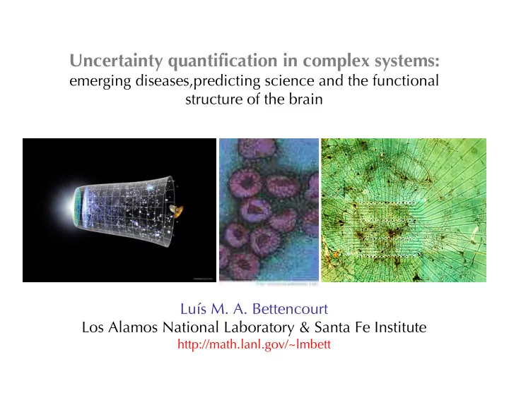
Uncertainty quantification in complex systems:

emerging diseases,predicting science and the functional structure of the brain Luís M. A. Bettencourt Los Alamos National Laboratory & Santa Fe Institute

http://math.lanl.gov/~lmbett

Uncertainty quantification in complex systems

Examples: climate, markets, cities, emerging diseases, science and innovation ecosystems and biodiversity, brain and cognition Properties: many components, heterogeneity, uncertainty in initial conditions and parameters, exposed to externalities, learn and adapt Modeling and theory in complex systems: No models exist that give long time predictability Few models have been proposed that give short term reliable predictions Causality is not well understood Uncertainty in models and predictions must be quantified for falsification Lots of data are coming in !

Synopsis

Predicting the epidemic potential of emerging infectious diseases with Ruy Ribeiro Accelerating Science and Technology with David Kaiser, OSTI DOE How do complex networks process information? the functional information structure of living neural networks with Vadas Gintautas and Michael Ham

Estimating the epidemic potential

• f emerging infectious diseases

“What’s the risk of a H5N1 (bird) flu pandemic in the next 3 years?” anonymous DHS program manager

October 1, 2004 March 23, 2005 May 19, 2005

time [days]

Outbreak of Marburg fever: Angola, 2005

Conditions in Uige:

“What’s the risk of a H5N1 (bird) flu pandemic in the next 3 years?” anonymous DHS program manager

H5N1 avian influenza

Influenza A virus, very contagious among birds: pandemic: Asia, Europe, Africa 51 countries Caused over 381 human cases, with 240 deaths 63% case mortality Presently very low transmissibility among humans: 0 < R0 << 1 How will H5N1 influenza evolve? What will be the signs of sustained human transmission: R0<1, R0 1?

Number of new cases induced by an infectious individual:

Typical EID time series

human cases of H5N1influenza in Vietnam

From “Situation Updates: Avian Influenza” Word Health Organization (WHO) Laboratory confirmed H5N1 cases (http://www.who.int/csr/don/en).

• vs. Seasonal flu epidemic time series

H3N2 USA isolates 2004-05

H3N2 seasonal influenza isolates from the Center for Disease Control (CDC) Surveillance Weekly Reports in the United States (http://www.cdc.gov/flu/weekly/fluactivity.htm)

Requirements for model of EID

i) incorporate reservoir sources, associated with multiple introductions ii) formulate the model in discrete probabilistic form iii) quantify uncertainty in epidemiological parameters and use new data to reduce it iv) cast state variables in terms of observable quantities, reported from field surveillance v) estimation procedure should not depend on future unknown data, such as final case cluster size vi) supply surveillance with real-time probabilistic expectations, which when violated may indicate that:

• there are errors in the new data
• the pathogen is evolving
• the host population is changing

A successful model for EID should:

Epidemic Mean Dynamics in terms of ‘observables’

SIR model without Sources

S

• = −β S

N I, I

• = β S

N − γ ⎡ ⎣ ⎢ ⎤ ⎦ ⎥ I

T

• = β S

N I

I(t + τ) = I(t)exp γ R0 S(t') N −1 ⎛ ⎝ ⎜ ⎞ ⎠ ⎟

t t +τ

∫

dt' ⎡ ⎣ ⎢ ⎤ ⎦ ⎥ ≅ I(t)exp γτ R0 S N −1 ⎛ ⎝ ⎜ ⎞ ⎠ ⎟ ⎡ ⎣ ⎢ ⎤ ⎦ ⎥

ΔT(t + τ) = b(R)ΔT(t)

Consider a standard SIR model: Total Cases: The solution is: Evolution of the expectation value for New Cases

b(R0) = exp γτ R0 S N −1 ⎛ ⎝ ⎜ ⎞ ⎠ ⎟ ⎡ ⎣ ⎢ ⎤ ⎦ ⎥

b(R) is the branching parameter: R0 = β/γ

RML = 1+ 1 γτ ln ΔT(t + τ) ΔT(t)

Epidemic time delay diagrams: R>1

R0 can be determined geometrically,

• without complex parameter estimation.

b(R) is the slope of the tangent at the origin

ΔT(t + τ) = b(R)ΔT(t)

Model with Sources

(multiple introductions)

Ih

• = β S(t)

N − γ ⎡ ⎣ ⎢ ⎤ ⎦ ⎥ Ih(t) + βbh S(t) N fcK(t), Ib

• = βbh

S(t) N (1− fc)K(t) − γIb

Model with two classes of human infected: Take: to give:

B

• = βbh

S(t) N K(t)

I

• = β S(t)

N − γ ⎡ ⎣ ⎢ ⎤ ⎦ ⎥ Ih(t) + B

• − γIb,

T =

• β S(t)

N Ih(t) + B

• .

Ih(t + τ) = b(R0) Ih(t) + e−γ(R0S / N−1) fc B

• (t')dt'

t t +τ

∫

⎡ ⎣ ⎢ ⎤ ⎦ ⎥ ≡ b(R0)) Ih(t) + fcψ(t,τ,B)

[ ]

Leading to the solution:

Model with Sources (cont.)

(multiple introductions)

ΔT(t + τ) = ΔB(t + τ) + b(R0) ΔT(t) − ΔB(t) + τγ R0 S N fcΔB(t) ⎡ ⎣ ⎢ ⎤ ⎦ ⎥

The progression of the expectation value for New Cases obeys: new cases from sources (birds) time evolution

• ld cases from

human transmission evolution of introduced infectious cases New cases are treated as a stochastic variable with this average

ΔT(t + τ) ~ P[ΔT(t + τ) ← ΔT(t) | Γ]

The functional form of P is constrained by the mean

Probabilistic Epidemic Models Real Time] Bayesian Parameter Estimation

Estimating the probability distribution of R, γ, etc from surveillance time series

is equivalent to: Alternative perspective: “Boundary value problem” Previous Cases + New Cases probability dist. of model (Γ) surveillance time series

P(Γ)

Usual perspective: “Initial value problem” Previous cases + Model (Γ) probability dist. of New Cases

This results from Bayes’ Theorem

• P[Γ] is the ‘prior’ [ it expresses the expected distribution of Γ]
• is a normalization factor:

P[Γ | ΔT(t + τ) ← ΔT(t)] = P[ΔT(t + τ) ← ΔT(t) | Γ]P[Γ] P[ΔT(t + τ) ← ΔT(t)]

P[ΔT(t + τ) ← ΔT(t)]

P[ΔT(t + τ) ← ΔT(t)] = dΓ

∫

P[ΔT(t + τ) ← ΔT(t) | Γ]P[Γ]

Γ are the model parameters

Iterative estimation and uncertainty reduction

P[Γ | ΔT(t + τ) ← ΔT(t)] = P[ΔT(t + τ) ← ΔT(t) | Γ]P[Γ] P[ΔT(t + τ) ← ΔT(t)]

At the next time At this time

Simulated Outbreaks

Real time evolution of maximum likelihood R0 and 95% confidence interval

H5N1 avian influenza: Vietnam H3N2 seasonal influenza: USA

θ=0.6

Indonesia

The R0 of H5N1 influenza in humans

VIETNAM INDONESIA Average fraction of cases attributable to human contagion (θ) 1.0 0.8 0.4 0.2 1.0 0.8 0.4 0.2 R0 min 0.26 0.23 0.68 0.56 0.26 ML R0 0.53 0.46 0.84 0.71 0.43 Mean R0 0.52 0.46 0.08 0.83 0.70 0.42 R0 max 0.77 0.68 0.46 0.97 0.83 0.56

even in worst case scenario: R0<1

Active surveillance through real time prediction and anomaly detection

Γ, ΔT(t)

ΔT(t + τ) ~ P[ΔT(t + τ) ← ΔT(t) | Γ]

anomalies Standard p-value test at 95% significance

Accelerating Science and technology

a predictive “science of science”?

Can science be forecast?

• when is a field opening or closing?
• what are the signatures of new scientific discoveries?
• “Paradigm shifts” vs. “normal science”

can they be distinguished from analysis of literature?

Prediction enables “interventions”:

How should agencies and institutions allocate resources: Students? Meetings? Individual PIs? How can scientific discovery be accelerated? NSF, DOE OSTI

The structure of scientific revolutions

“normal science” “paradigm shift” discovery invention crisis “exceptional science”

• T. Kuhn 1961

[puzzle solving] […] time dissolution [discovery & invention] inconsistencies Are there quantitative signatures

• f where a field is ?

6+2 examples of scientific discovery

Cosmological Inflation Cosmic Strings String Theory Prions H5N1 Influenza Quantum Computing & Computation Carbon Nanotubes Cold Fusion

Theoretical Physics BioMedical Applied Physics Material Science Engineering “Pathological” Science

Data sources and retrieval

SearchPlus developed by the LANL’s Research Library Library Without Walls (http://library.lanl.gov/lww/) Searches the standard set of largest scientific databases: BIOSIS Engineering Index Proceedings Inspec ISI databases (Thomson Scientific): ISI Proceedings ISI SciSearch ISI Social SciSearch ISI Arts & Humanities Retrieved data (HTML) -> Parsed -> Relational Databases authors, title, date, journal reference

Each field is built from a combination of searches and analyzed by a domain expert

Ideas as ‘epidemics of knowledge’

Parallels between social dynamics and epidemiology

Individual Susceptible Exposed Infectious Recovered Social (population)

Host/pathogen dynamics

subpopulation in classes contact rate incubation time infectious period

no intentionality in standard disease contagion

Dynamical Model

dS dt = Λ − βS I N , dE dt = βS I N − ρS I N −κE, dI dt = ρS I N +κE − γI, dR dt = γI

R0=β/γ is a measure of transmissibility Basic reproduction number

Strategy:

• Search for the best parameters is an optimization

problem: minimizing the deviation of the model relative to the data

• Optimization within a fixed tolerance leads to many

good solution from which we construct: Joint probability distribution for model parameters conditional

• n observed data:

P[Γ I O ] Γ = (S(t0),I(t0),E(t0),R(t0),β,Λ,κ,ρ,γ )

Initial State Dynamical Parameters

Parameter Search and Optimization

Indirect estimation of from trajectories:

Deviation (action): where IΓ(ti) is the state given by solving the model with initial conditions and dynamical parameters given by Γ, evaluated at the data points Inverse Problem Thus we can associate a (goodness of fit) probability for the trajectory IΓ(t) as

P[Γ I O ]

A(Γ) = 1 N

I Γ (ti )−I O (ti )

( )

2σ ti i=1 N

∑

2

wΓ =

1 Nw e−AΓ , Nw = Tr[wΓ]

Cosmological Inflation

[2005: 3410 authors, 5135 papers] Alan Guth 1981 Andrei Linde 1982 Proposes Explanations for many cosmological problems: Boosted by recent Cosmic Microwave Background Measurements

Cosmic Strings and Topological Defects

[2005: 2292 authors; 2443 authors] TWB Kibble 1976 Y Zeldovich 1980 Unavoidable features of the Early Universe: Could they have seeded structure? Disfavored by Current CMB measurements

Scrapie and Prions

[2005:14620 authors, 11074 papers] Prussiner 1982 Nobel Prize 1997 Misfolding Proteins that cause transmissible spongiform encephalopathies: Scrapie, “mad cow disease” Kreuzberg-Jacob disease in humans

H5N1 Influenza (bird flu)

[2005:1281 authors, 604 papers] Disease of birds First infected humans in 1997 in Hong Kong 280 humans infected ~60% case mortality

Carbon Nanotubes

[2005: 25464 authors, 30521 papers]

• S. Ijima 1992

Important subfield

• f nanotech

Allotrope of Carbon Promises to revolutionize Nano-engineering

Quantum Computers and Computation

[2005: 7518 authors; 8946 papers] First references 1960s-70s Feynman 1982 Deutsch 1985 Algorithms: Shor, Grover ~1995 NMR Experiments ~1996 Revolution in Computing & Cryptography?

Cold Fusion

pathological science

[2005: 1637 authors; 871 papers]

Utah experiments

Estimated parameters

infectiousness and recruitment pull of scientific ideas

Measures of Scientific Productivity

Marginal Returns

ΔY(t') ΔX(t) = f [ΔX(t)] ~ [ΔX(t)]β, t'≥ t

Output Input scaling relation (?) “Returns to Scale” in ΔY=Papers versus ΔX=Authors: citations, patents funding, reputation β=1 : each unit of input produces one unit of output β <1 : diminishing returns: each new author -> less papers/author β >1 : increasing returns: each new author -> more papers/author

Theoretical Physics

Cosmological Inflation β=1.28 Cosmic Strings β=1.13

BioMedical Fields

Prions β=0.78 H5N1 Influenza β=0.87

Technological Fields

Carbon Nanotubes β=1.32 Quantum Computation β=1 vs. 1.37

Science may be forecast uncertainty quantification in predictions is essential for model building and falsification

Information processing in the nervous system

functional information modules in complex networks

Mouse liver gene expression network from Jake Lusis Laboratory,UCLA

Functional subgraphs

Curse of dimensionality

motifs

Entropy as uncertainty Mutual Information as uncertainty reduction

Shannon Entropy of X:

S(X) = − p(x)log2

x

∑

p(x)

S(X;Y) = S(X) + S(Y) + I(X;Y)

Shannon Entropy of {X;Y}:

I(X;Y) = p(x,y)log2

x,y

∑

p(x,y) p(x)p(y) ⎛ ⎝ ⎜ ⎞ ⎠ ⎟

Mutual Information {X;Y}:

measures correlation between states of X;Y measures number of states of X; stochasticity

A [discrete] calculus in information

measurement and information gain

A cluster decomposition in terms of functional modules

Rn gives redundancy or synergy exactly to nth order

Frontal cortex neurons from fetal mice [thousands/mm2] Grown in vitro over a 1mm2 microelectrode array Disassociated Culture spontaneously form network

Image courtesy M. Ham and G. Gross

Architecture and information processing in the nervous system

Cortical neural network electrophysiological activity

Estimation in practice

Binary ‘words’ from spike time series

“Spikes” Rieke, Warland, de Ruyter van Steveninck, Bialek

And count word frequencies over time

pw = nw N

Motif search and identification

• ptimization in uncertainty reduction

Approximate searches

Reverse engineering network circuits

Randomness or Structure?

Individual uncertainty is accounted for by other nodes

Uncertainty in models of complex systems

Uncertainty quantification and management

is essential in complex systems no [exact] predictive models exist many uncertainties in initial conditions and parameters exogenous shocks

Uncertainty reduction via optimization reveals

the functional network structure of complex systems as information processing systems generates robust adaptive control protocols, active learning and recovery