U a + b " 2 2 a b " 1 a b 2 p Figure: - PowerPoint PPT Presentation

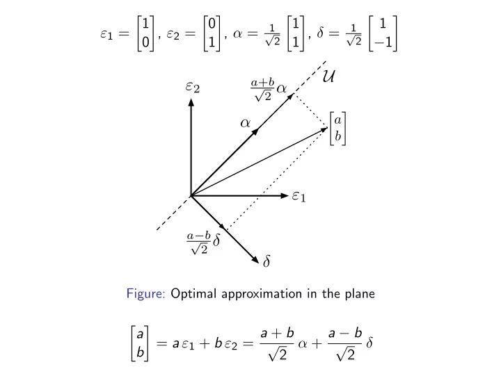
� 1 � 1 � � 0 � � 1 � � 1 1 ε 1 = , ε 2 = , α = , δ = √ √ 0 1 1 − 1 2 2 U a + b " 2 2 α √ � � a α b " 1 a − b 2 δ p δ Figure: Optimal approximation in the plane � a � = a ε 1 + b ε 2 = a + b α + a − b √ √ δ b 2 2

Another basis for V = L 2 ([0 , 1)) ◮ Use step functions for approximation! ◮ This allows for ◮ capturing local properties of functions ( localization ) ◮ refinement by adjusting the step width ( resolution ) The relevant operations are known as translation and dilation ◮ Two basic scaling operations for functions f : R → C , in particular for f ∈ L 2 ( R ) ◮ dilation: for a > 0 ( D a f )( t ) = √ a f ( a t ) ◮ translation: for b ∈ R ( T b f )( t ) = f ( t − b )

Illustration of Dilation and Translation (1) 1.0 0.5 - 2 - 1 1 2 3 4 5 - 0.5 - 1.0 Figure: The function f ( t ) = sin( t 2 ) · 1 [0 , 3 π ) ( t ) 1.0 0.5 - 2 2 4 6 - 0.5 - 1.0 Figure: The functions f ( t ) (black), T 2 f ( t ) (green), T − 2 f ( t ) (blue)

Illustration of Dilation and Translation (2) 1.0 0.5 - 2 - 1 1 2 3 4 5 - 0.5 - 1.0 Figure: The function f ( t ) = sin( t 2 ) · 1 [0 , 3 π ) ( t ) 1.5 1.0 0.5 2 4 6 - 0.5 - 1.0 - 1.5 Figure: The functions f ( t ) (black), D 1 / 2 f ( t ) (green), D 2 f ( t ) (blue)

Illustration of Dilation and Translation (2) 1.0 0.5 - 2 - 1 1 2 3 4 5 - 0.5 - 1.0 Figure: The function f ( t ) = sin( t 2 ) · 1 [0 , 3 π ) ( t ) 1.5 1.0 0.5 2 4 6 - 0.5 - 1.0 - 1.5 Figure: The functions f ( t ) (black), D 1 / 2 f ( t ) (green), D 2 f ( t ) (blue)

Illustration of Dilation and Translation (3) 1.5 1.0 0.5 - 1 1 2 3 4 - 0.5 - 1.0 - 1.5 Figure: The functions T 2 D 2 f ( t ) (green) and D 3 / 2 T − 1 ( t ) (blue) 1.5 1.0 0.5 - 1 1 2 3 4 - 0.5 - 1.0 - 1.5 Figure: The functions T 1 D 1 / 2 f ( t ) (green), D 1 / 2 T 1 f ( t ) (blue)

Properties of Dilation and Translation ◮ Check! 1. D a ( D b f ) = D a · b f 2. T a ( T b f ) = T a + b f 3. D a ( T b f ) = T b / a ( D a f ) 4. � f | D a g � = � D 1 / a f | g � 5. � f | T b g � = � T − b f | g � 6. � D a f | D a g � = � f | g � , in particular � D a f � = � f � 7. � T b f | T b g � = � f | g � , in particular � T b f � = � f �

The Haar scaling function ◮ For an interval I = [ a , b ) ⊂ R its indicator function is � 1 if a ≤ t < b 1 I ( t ) = 1 [ a , b ) ( t ) = 0 otherwise Similarly for intervals [ a , b ] or ( a , b ] or ( a , b ) ◮ The dyadic itervals I j , k (for j , k ∈ Z ) are defined as I j , k = [ k · 2 − j , ( k + 1) · 2 − j ) ◮ The Haar scaling function is defined as � if 0 ≤ t < 1 1 φ ( t ) = 1 I 0 , 0 ( t ) = 1 [0 , 1) ( t ) = 0 otherwise ◮ For j , k ∈ Z put φ j , k ( t ) = ( D 2 j T k φ )( t ) = 2 j / 2 · φ (2 j t − k ) = 2 j / 2 1 I j , k ( t ) ◮ j : dilation parameter ( resolution ), ◮ k : translation parameter ( localization )

Properties of the φ j , k ◮ Orthogonality � � φ j , k | φ j ,ℓ � = φ j , k ( t ) φ j ,ℓ ( t ) dt = δ k ,ℓ R ◮ That is: for any fixed j ≥ 0 the family Φ j = { φ j , k ( t ) ; 0 ≤ k < 2 j } is an orthonormal system in L 2 ([0 , 1)) ◮ The subspace V j of V = L 2 ([0 , 1)) generated by taking Φ j as its basis is the space of dyadic step functions with step width 2 − j The space V j has dimension 2 j This space is known as approximation subspace on level j ◮ The scaling equation relates V j and V j +1 1 √ φ j , k ( t ) = ( φ j +1 , 2 k ( t ) + φ j +1 , 2 k +1 ( t )) 2

Illustrations of the Haar scaling function 1.0 0.8 0.6 0.4 0.2 - 1.0 - 0.5 0.5 1.0 1.5 2.0 Figure: The Haar scaling function φ ( t ) 2.5 2.0 1.5 1.0 0.5 - 2 - 1 1 2 3 Figure: φ 1 , 1 ( t ) (black), φ 2 , − 3 ( t ) (red), φ 3 , 10 ( t ) (green), φ − 1 , 0 ( t ) (blue)

Optimal approximation with step functions ◮ Optimal approximation in V j for f ∈ L 2 ([0 , 1)) � α j ( f ; t ) = a j , k φ j , k ( t ) 0 ≤ k < 2 j has approximation coefficients � a j , k = � f | φ j , k � = 2 j / 2 f ( t ) dt I j , k ◮ Important: unlike the Fourier coefficients, the approximation coefficients a j , k only depend locally on f ( t ), precisely: a j , k · φ j , k ( t ) = µ j , k ( f ) · 1 I j , k ( t ) , 1 � where µ j , k ( f ) = f ( t ) dt | I j , k | I j , k is the average of f ( t ) over I j , k

Changing the resolution ◮ Important question: how do the approximation coefficients a j , k change when changing the resolution parameter j ? ◮ Partial answer: from I j , k = I j +1 , 2 k ⊎ I j +1 , 2 k +1 it follows that � a j , k = 2 j / 2 f ( t ) dt I j , k � � = 2 j / 2 ( f ( t ) dt + f ( t ) dt ) I j +1 , 2 k I j +1 , 2 k +1 = 2 ( j +1) / 2 � � √ ( f ( t ) dt + f ( t ) dt ) 2 I j +1 , 2 k I j +1 , 2 k +1 1 √ = ( a j +1 , 2 k + a j +1 , 2 k +1 ) 2

Changing the resolution ◮ The recurrence equation for the Haar approximation coefficients 1 √ a j , k = ( a j +1 , 2 k + a j +1 , 2 k +1 ) 2 is really a consequence of the scaling equation 1 φ j , k ( t ) = √ ( φ j +1 , 2 k ( t ) + φ j +1 , 2 k +1 ( t )) , 2 because by linearity of the inner product 1 � f | φ j , k � = √ ( � f | φ j +1 , 2 k � + � f | φ j +1 , 2 k +1 � ) 2

Changing the resolution ◮ The complete answer: ◮ Define detail coefficients for 0 ≤ k < 2 j 1 d j , k = √ ( a j +1 , 2 k − a j +1 , 2 k +1 ) 2 then � � a j +1 , 2 k � a j , k � 1 � 1 � 1 √ = 1 − 1 d j , k a j +1 , 2 k +1 2 and consequently � a j +1 , 2 k � 1 � 1 � � a j , k � 1 = √ a j +1 , 2 k +1 1 − 1 d j , k 2 ◮ This defines the Haar transformation at level j + 1! ( a j +1 , 0 , a j +1 , 1 , . . . , a j +1 , 2 j +1 − 1 ) � ( a j , 0 , a j , 1 , . . . , a j , 2 j − 1 , d j , 0 , d j , 1 , . . . , d j , 2 j − 1 )

What the d j , k really are ◮ From the definition: 1 √ d j , k = ( a j +1 , 2 k − a j +1 , 2 k +1 ) 2 = 2 ( j +1) / 2 � � √ ( f ( t ) dt − f ( t ) dt ) 2 I j +1 , 2 k I j +1 , 2 k +1 = � f | ψ j , k � ψ j , k ( t ) = 2 j / 2 ψ (2 j t − k ) where and where  1 f¨ ur 0 ≤ t < 1 / 2   ψ ( t ) = 1 [0 , 1 / 2) ( t ) − 1 [1 / 2 , 1) ( t ) = − 1 ur 1 / 2 ≤ t < 1 f¨  0 sonst  is known as the Haar wavelet function ◮ Note that ψ j , k ( t ) = ( D 2 j T k ψ )( t )

Illustration of the Haar wavelet function 1.0 0.5 - 2 - 1 1 2 3 - 0.5 - 1.0 Figure: The Haar wavelet function ψ ( t ) 3 2 1 - 1.0 - 0.5 0.5 1.0 1.5 2.0 - 1 - 2 - 3 Figure: ψ 1 , 1 ( t ) (black), ψ 2 , − 3 ( t ) (red), ψ 3 , 10 ( t ) (green) ψ − 1 , 0 ( t ) (blue)

The wavelet equation appears ◮ The definition of the d j , k is equivalent to the wavelet equation 1 √ ( φ j +1 , 2 k ( t ) − φ j +1 , 2 k +1 ( t )) ψ j , k ( t ) = 2 ◮ The family Ψ j = { ψ j , k ( t ) } 0 ≤ k < 2 j is an ONS in V = L 2 ([0 , 1)) ◮ The subspace W j of V = L 2 ([0 , 1)) generated by Ψ j is called wavelet or detail subspace at level j ◮ The space W j has dimension 2 j ◮ Check: All φ j , k are orthogonal to all ψ j ′ ,ℓ for j ≤ j ′ and (0 ≤ k < 2 j , 0 ≤ ℓ < 2 j ′ ) ◮ Check: All ψ j , k are orthogonal to all ψ j ′ ,ℓ for j ′ � = j

Putting φ and ψ together ◮ The functions Φ j +1 = { φ j +1 , k ( t ) } 0 ≤ k < 2 j +1 generate (as an ONS) the subspace V j +1 of V = L 2 ([0 , 1)) of step functions of step width 2 − j − 1 This space has dimension 2 j +1 ◮ By definition V j ⊂ V j +1 and W j ⊂ V j +1 ◮ But the space V j +1 also has Φ j ∪ Ψ j = { φ j , k ( t ) } 0 ≤ k < 2 j ∪ { ψ j , k ( t ) } 0 ≤ k < 2 j as an ONS! Hence V j +1 = V j ⊕ W j

Two bases in one space ◮ The 1-level Haar transformation (at level j + 1) is an orthogonal basis transformation in the space V j +1 between bases Φ j +1 and Φ j ⊕ Ψ j ◮ which explicitly reads � � φ j +1 , 2 k ( t ) � φ j , k ( t ) � � 1 � 1 1 = √ ψ j , k ( t ) 1 − 1 φ j +1 , 2 k +1 ( t ) 2 and equivalently � φ j +1 , 2 k ( t ) � 1 � 1 � � φ j , k ( t ) � 1 √ = − 1 φ j +1 , 2 k +1 ( t ) 1 ψ j , k ( t ) 2

Basic identities ◮ Haar scaling identity (Analysis) 1 √ φ j , k ( t ) = ( φ j +1 , 2 k ( t ) + φ j +1 , 2 k +1 ( t )) 2 ◮ Haar wavelet identity (Analysis) 1 √ ψ j , k ( t ) = ( φ j +1 , 2 k ( t ) − φ j +1 , 2 k +1 ( t )) 2 ◮ Both identities together (Analysis) � � φ j +1 , 2 k ( t ) � φ j , k ( t ) � 1 � 1 � 1 √ = ψ j , k ( t ) 1 − 1 φ j +1 , 2 k +1 ( t ) 2 ◮ Reconstruction (Synthesis) � φ j +1 , 2 k ( t ) � 1 � 1 � � φ j , k ( t ) � 1 √ = − 1 φ j +1 , 2 k +1 ( t ) 1 ψ j , k ( t ) 2

Transforming the coefficients ◮ Analysis � � a j +1 , 2 k � a j , k � 1 � 1 � 1 = √ 1 − 1 d j , k a j +1 , 2 k +1 2 ◮ Synthesis � a j +1 , 2 k � 1 � 1 � � a j , k � 1 √ = 1 − 1 a j +1 , 2 k +1 d j , k 2 ◮ This defines the Haar transformation at level j + 1! ( a j +1 , 0 , a j +1 , 1 , . . . , a j +1 , 2 j +1 − 1 ) � ( a j , 0 , a j , 1 , . . . , a j , 2 j − 1 , d j , 0 , d j , 1 , . . . , d j , 2 j − 1 )