Tuesday, June 18, 2013 1 pm 2:30 pm PST 2 pm 3:30 pm MST 3 pm - - PowerPoint PPT Presentation

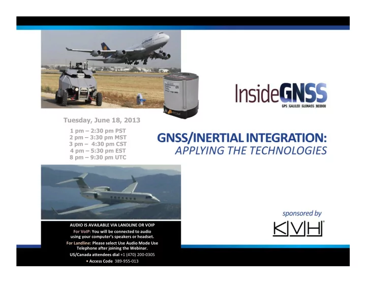
1 pm – 2:30 pm PST 2 pm – 3:30 pm MST 3 pm – 4:30 pm CST 4 pm – 5:30 pm EST 8 pm – 9:30 pm UTC

Tuesday, June 18, 2013

AUDIO IS AVAILABLE VIA LANDLINE OR VOIP For VoIP: You will be connected to audio using your computer’s speakers or headset. For Landline: Please select Use Audio Mode Use Telephone after joining the Webinar. US/Canada attendees dial +1 (470) 200-0305

• Access Code 389-955-013

WELCOME TO:

GNSS /Inertial Integration: Applying the Technologies

Moderator: Mark Petovello, Geomatics Engineering, University of Calgary, Contributing Editor at Inside GNSS Co-Moderator: Mike Agron, Executive Webinar Producer

Audio is available via landline or VoIP For VoIP: You will be connected to audio using your computer’s speakers or headset. For Landline: Please select Use Audio Mode Use Telephone after joining the Webinar. US/Canada attendees dial +1 (470) 200-0305 Access Code: 389-955-013

Andrey Soloviev

Principle Qunav

Xavier Orr

Lead Software Engineer Advanced Navigation Pty Ltd

Who’s In the Audience?

15% Professional User 19% GNSS Equipment Manufacturer 19% Product / Application Designer 22% System Integrator 25% Other

A diverse audience of over 700 professionals registered from 59 countries, 31 states and provinces representing the following roles:

How to ask a question

Poll

Post-webinar survey

Recording

Housekeeping Tips

Welcome from Inside GNSS

Richard Fischer Director of Business Development Inside GNSS

A word from the sponsor

Jay Napoli Vice-President, FOG & OEM Sales KVH Industries, Inc.

GNSS/Inertial Integration

Mark Petovello Geomatics Engineering University of Calgary Contributing Editor Inside GNSS

Today: “Applying the Technologies”

• Trends
• Key challenges
• Applications
• Beyond GNSS/INS
• And more…

The GNSS/INS Webinar Series to Date

Dec ′09: “Nuts & Bolts”

• Key inertial equations
• Integration concepts & equations
• Demonstrate possible results

Feb ′12: “Filling in the Gaps”

• Select an integration strategy
• Practical considerations
• Sensor characterization

Past webinars available at: http://insidegnss.com/webinars

What would you say is the greatest challenge with

integrating GNSS/INS? (select one)

1.

Modeling the inertial errors

2.

Identifying good/bad GNSS data

3.

How to integrate other sensor data

4.

Selecting architectures for GNSS/INS integration

Poll #1

Featured Presenter

Andrey Soloviev

Principle Qunav

Andrey Soloviev Principle Qunav

Technology Overview

Combination of complementary features of GNSS and Inertial

Integration of self-contained but drifting inertial with GNSS that is drift-less but susceptible to interference

Wide range of GNSS/Inertial products

Examples:

• Embedded GPS/INS (EGI) for military applications

Limitations: Use of relatively high grade, expensive inertial units

• GNSS/Inertial products for ground and aerial applications

Limitations: Some designs have limited capabilities in GPS denied environments

Current Status

Development Trends

From open-sky environments to urban canyons, indoors and underwater From GNSS/INS to INS/GNSS+ From high-grade inertial products to low-cost sensors (e.g., consumer-grade) INS INS

Motion constraints

What is the Right Integration Approach

Tight and deep integration are more suitable for GNSS-challenged environments and integration of inertial with other sensors

• Loose Integration: Fusion of navigation solutions
• Tight Integration: Fusion of navigation measurements
• Deep Integration: Integration at the signal processing level

Loose integration has limited capabilities in GNSS-challenged environments

Example: sparse GNSS position fixes in urban canyon Some data may be still available (e.g. 2-3 satellites) for tight and deep modes No GNSS data for loose integration

Data Fusion Tools

GNSS/Inertial: Complementary Extended Kalman Filter INS/GNSS+: Kalman filter is not necessarily the best option and the use of nonlinear filtering techniques may be required

Example: A constraint that the platform stays within the hallway can be directly incorporated using particle filters

Assumptions:

• Linear system model;
• Gaussian error distribution

Featured Presenter

Xavier Orr

Lead Software Engineer Advanced Navigation Pty Ltd

Xavier Orr Lead Software Engineer Advanced Navigation Pty Ltd

Introduction

Aim to produce inertial navigation system with

superior dead reckoning

Advanced north seeking capability Price target of under USD 30,000

Orientation Accuracy

For long term dead reckoning, highly accurate orientation

is essential

Orientation is tracked from gyroscopes and corrected for

errors from gravity vector and other sources

Orientation Accuracy

High accuracy gyroscopes with very high bias stability are

essential to maintain orientation accuracy

Accelerometers with high bias stability are essential to

provide a reference for the level orientation (gravity vector)

Heading is more complicated Gravity Vector X Pitch Gravity Vector Y Roll Z Z

Heading

• Possible sources of heading are GNSS velocity, magnetometers,

north seeking gyro-compassing and external references

• Magnetometers and north seeking gyro-compassing are the only

always available sources

Magnetic Heading

Magnetic heading is prone to interference, particularly in

today's high tech environments

Magnetic heading is not good for a high accuracy absolute

reference, but good for a relative reference

North Seeking Heading

Gyroscopes can detect the earth rotation rate Have to separate earth rotation from gyroscope bias, noise and

• ther error sources

Accurate north seeking gyro-compassing requires high bias

stability gyroscopes

Commercially Available IMUs

After market research KVH Industries 1750 IMU found to

provide best commercial gyroscopes available

Excellent gyroscope bias stability of 0.05 degrees/hour well

suited to provide high accuracy orientation and north seeking

Very low bias accelerometers in 1750 allows for fast

initialization

Andrey Soloviev Principle Qunav

• Motivation: INS is a dead-reckoning solution that needs to be initialized
• Position and velocity initialization is straightforward when GNSS is available
• How to initialize the attitude?

Initial Alignment: Attitude Initialization

We need two know projections of two non-collinear vectors (A and B) in navigation- frame and INS body-frame Then find a rotation that aligns body-frame and navigation-frame vectors’ projection

Cb

N

A B xN yN zN A B xb yb zb xb yN zN xb yb zb xN yb zb

Cb

N

• Step 1: Align vector A

Alignment Sequence

A xN yN zN A xb yb zb Computationally rotate body-frame such that projections of vector A are aligned with its navigation-frame projections xb yb zb After that, body-frame is still not completely aligned with the navigation frame as there is a rotational degree

• f freedom around vector A

Body-frame view xb yb zb Abefore Aafter

Rotation angle Rotation axis

C1

• Step 2: Align vector B

Alignment Sequence

Computationally rotate body-frame (from its new orientation) around vector A such that projections of vector B are aligned with its navigation-frame projections A xb yb zb

C2

B xb yN zN xN yb zb

Cb

N = C2⋅ C1

Initial orientation

• Classical approach
• Alternative approach for lower-grade inertial sensors

Initial Alignment: Which Two Vectors To Use?

Vector 1: Acceleration due to gravity:

• Known in navigation-frame (gravitational model);
• Measured in body-frame (accelerometers)

Vector 2: Earth rate:

• Known in navigation-frame (based on initial position);
• Measured in body-frame (gyros)

Requires high-grade gyros since the Earth rate is 15 deg/hr

Vector 2: Velocity vector:

• Navigation-frame: measured by GNSS;
• Body-frame: assumed to be aligned with

the front axis of the vehicle

x z y

V

Another option: use of magnetometers

Use of Motion Constraints: General Approach

Use as additional measurement(s) for the complementary Kalman filter

f( ˆ R

INS, ˆ

V

INS, ˆ

α α α α

INS,ˆ

a

INS, ˆ

w

INS)

INS-predicted value: Linearize (inertial errors generally

allow for linearization)

Kalman filter estimation update Estimates of INS drift terms

f(R,V,α α α α,a,w) = 0

Motion constraint (which is generally a non-linear function of navigation and motion states)

Use of Motion Constraints: Example

Automotive application

Zero cross-track velocity

Vy b = 0

1

[ ]⋅ ˆ

C

N b ⋅ ˆ

V

INS

Motion constraint Linearization Kalman filter measurement observable

Coordinate transformation from navigation into body frame Projection on yb-axis

1

[ ]⋅ ˆ

C

N b ⋅ δVINS + 0

1

[ ]⋅ ˆ

C

N b ⋅ VINS × δθ

θ θ θINS

Velocity error Attitude error Cross product

xb zb yb

Andrey Soloviev

Principle Qunav

Xavier Orr

Lead Software Engineer Advanced Navigation Pty Ltd

Jay Napoli

Vice-President, FOG & OEM Sales KVH Industries, Inc.

Ask the Experts – Part 1

Poll #2

Which types of IMU technologies have you had the MOST experience with? (Choose One)

• 1. MEMS
• 2. RLG (Ring-laser Gyros)
• 3. FOG (Fiber Optic Gyros)
• 4. Electro-mechanical
• 5. Not sure or none

Xavier Orr Lead Software Engineer Advanced Navigation Pty Ltd

Spatial FOG Finished Integrated Product

Sensors

Gravity Vector Reference Motion Analysis Body Acceleration Gyroscopes Accelerometers Angular Velocity North Seeking Gyrocompass Motion Analysis Magnetometers Speed up initial heading alignment Zero yaw rate updates help track gyroscope bias

Sensors

GNSS Barometric Pressure Position, velocity and time Carrier phase delta updates Odometer Pulse Period Average Velocity Pulse Count Distance Update Vertical velocity stabilization Other Sensors Velocity, Speed or Zero Velocity Updates Position updates

Filter

Multiple simultaneous correction sources used Filter tracks history of correction standard deviation

and predicts future correction standard deviation

Attitude corrections based on gravity vector can

introduce error

To reduce this, the filter predicts and compensates for

linear accelerations

Balancing inertial bias tracking and north seeking is

the biggest challenge

Magnetometers

Automatic magnetic calibration Magnetometers speed up north seeking initialization During operation magnetometers used primarily for zero

yaw rate updates to assist in tracking Z axis gyroscope bias

This makes the system immune to magnetic interference

GNSS

GNSS provides position, velocity and time during

normal operation

When a fix is not possible carrier phase delta is used

for velocity updates

Tightly coupled but completely GNSS independent

architecture

RTK available for applications requiring high accuracy

positioning

RAIM FDE for safe operation

Motion Analysis

Analyses patterns in inertial data Zero velocity updates Zero yaw rate updates Speed prediction for forward driving vehicles under GNSS

• utages

Hot Start

Previous position, velocity, heading and bias model

retained for very fast INS start

Time tracked with RTC Almanac, ephemeris, position and time sent to GNSS

receiver for hot start

Hot start allows for high accuracy orientation quickly Ideal for vehicles that don't move when powered down Fast recovery from power outages

Timing & Update Rate

Timing is critical for INS High update rate reduces integration and other errors

but requires a lot of computing power and careful balancing of resources

To achieve this we designed our own safety oriented

real time operating system

Direct Memory Access (DMA) is the key to balancing

resources and achieving accurate timing

Powerful processor with Floating Point Unit and lots

• f RAM required

External Data

Delay estimation Standard deviation estimation External navigation aids

• Local RF positioning systems
• Rangefinders (Laser, ultrasonic, IR)
• RFID position tags
• WiFi
• Vision and stereo vision
• Stereo audio
• SLAM

Land, Air & Marine Applications

Navigation through GNSS outages and jamming Navigation in tunnels, indoor environments and

around structures obstructing satellite view

Beneficial for aircraft to maintain navigation through

rolls that can cause degraded GNSS visibility

Safety conscious autonomous vehicles

Subsea Applications

Subsea versions specially designed and optimized for

underwater navigation

High level of motion constraints allows for superior

navigation performance underwater

Andrey Soloviev Principle Qunav

Generic Integration Approach

• INS is a core sensor;
• Other sensors provide reference data (when available) to reduce drift in inertial

navigation outputs

Example Case Study 1

• How to extend GNSS/INS integration principles to include other sensors?
• Example: Integration of inertial and GNSS carrier phase

Temporal phase changes are applied as measurement observables of the Kalman filter to eliminate integer ambiguities

∆ϕ = ϕ(tn) - ϕ(tn-1)=∆ρ + ∆δtrcvr + η

− e,∆R

( )

Delta position or position change

Represented in a generic format:

∆ϕ = Hproj∆R + Dprojb +η

Bias states Projection matrices

Example Case Study 2

Odometer

Position change projected onto forward axis

2D lidar

Position change projected onto x and y axes of the body- frame Position change projected

• nto a normal vector of a

planar surface extracted from lidar image

xb yb zb ∆R xb yb zb ∆R ∆R n 3D lidar The same generic format can be applied for integration with other sensors whose measurements are related to position change (∆R) The integration software can fully utilize GNSS/INS development results, the developer just needs to select different projection matrices.

Non-Linear Filtering Techniques

• Extension of the EKF to support non-linear aiding measurements:

Example: Map-matching (hallway layout, Wi-Fi fingerprinting)

• For integration with INS, the extension is based on a marginalized particle filter (MPF):
• The estimation space is partitioned into linear and non-linear sub-spaces;
• Optimal EKF estimation is applied for the linear sub-space;
• Monte-Carlo approximation (a.k.a particle filter) is used for the non-linear sub-space;

Initial particles states (e.g. position states) are sampled from an a priory pdf Particle states and their EKF covariances are propagated using INS When aiding measurements arrive:

• Particle weights are updated (likelihood
• f the particle given the measurement);
• For each particle, EKF state vector and

covariance are updated

Example Simulation Results

• Integration of low-cost MEMS inertial, Vision, partial GPS (2 visible SVs) and a hallway layout

Performance of the marginalized particle filter

148 150 152 154 156 158 160 150 155 160 165 X, m Y, m

50 100 150 200 20 40 60 80 100 120 140 160 180 200 X, m Y, m

Initial distribution of particles

20 40 60 80 100 120 140 160 180 20 40 60 80 100 120 140 160 180 200 X, m Y, m

Particle distribution after 4 seconds zoom

True position

Poll #3

What challenges, if any, have you experienced with IMU technology? (Select all that apply)

• 1. Performance/accuracy limitations
• 2. Data communications
• 3. Size or weight
• 4. Interface connection issues
• 5. None

Next Steps Contact Info:

• For more information visit:

www.kvh.com/1750imu

• Email specific questions to: Sean McCormack: smccormack@kvh.com

For more information:

• Visit www.insidegnss.com/webinars for:
• PDF of Presentation
• List of resources provided

Ask the Experts – Part 2

Andrey Soloviev

Principle Qunav

Xavier Orr

Lead Software Engineer Advanced Navigation Pty Ltd

Jay Napoli

Vice-President, FOG & OEM Sales KVH Industries, Inc.

A word from the sponsor

www.kvh.com Name Organization Title Jay Napoli Vice-President, FOG & OEM Sales KVH Industries, Inc.

Thank You!

Andrey Soloviev

Principle Qunav

Xavier Orr

Lead Software Engineer Advanced Navigation Pty Ltd

Jay Napoli

Vice-President, FOG & OEM Sales KVH Industries, Inc.

Andrey Soloviev

Principle Qunav

Xavier Orr

Lead Software Engineer Advanced Navigation Pty Ltd

Jay Napoli

Vice-President, FOG & OEM Sales KVH Industries, Inc.