TSP: operational semantics / department of mathematics and computer - - PowerPoint PPT Presentation

SLIDE 1

/ department of mathematics and computer science

Process Algebra (2IMF10)

Theory of Sequential Processes Bas Luttik

MF 6.072 s.p.luttik@tue.nl http://www.win.tue.nl/~luttik

Lecture 5

2/15 / department of mathematics and computer science

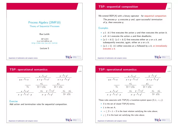
TSP: sequential composition

We extend BSP(A) with a binary operator · for sequential composition: The process p · q executes p and, upon successful termination

• f p, then executes q.

Examples

▶ a.1 · b.1 fjrst executes the action a and then executes the action b; ▶ a.0 · b.1 executes the action a and then deadlocks; ▶ (a.1 + b.1) · (a.1 + b.1) fjrst executes either an a or a b, and

subsequently executes, again, either an a or a b;

▶ (a.1 + 1) · b.1 either executes an a followed by a b, or immediately

executes a b.

3/15 / department of mathematics and computer science

TSP: operational semantics

a.x

a

− → x x

a

− → x′ x + y

a

− → x′ y

a

− → y′ x + y

a

− → y′ 1↓ x↓ (x + y)↓ y↓ (x + y)↓ x

a

− → x′ x · y

a

− → x′ · y x↓ y

a

− → y′ x · y

a

− → y′ x↓ y↓ (x · y)↓

Exercise

Add action and termination rules for sequential composition.

4/15 / department of mathematics and computer science

TSP: operational semantics

a.x

a

− → x x

a

− → x′ x + y

a

− → x′ y

a

− → y′ x + y

a

− → y′ 1↓ x↓ (x + y)↓ y↓ (x + y)↓ x

a

− → x′ x · y

a

− → x′ · y x↓ y

a

− → y′ x · y

a

− → y′ x↓ y↓ (x · y)↓

These rules associate with TSP(A) a transition-system space (S, L, →, ↓):

▶ S is the set of closed TSP(A)-terms; ▶ L is the set A; ▶ → ⊆ S × L × S is the least relation satisfying the rules above; ▶ ↓ ⊆ S is the least set satisfying the rules above.

SLIDE 2

5/15 / department of mathematics and computer science

TSP: operational semantics

a.x

a

− → x x

a

− → x′ x + y

a

− → x′ y

a

− → y′ x + y

a

− → y′ 1↓ x↓ (x + y)↓ y↓ (x + y)↓ x

a

− → x′ x · y

a

− → x′ · y x↓ y

a

− → y′ x · y

a

− → y′ x↓ y↓ (x · y)↓

Exercise

Compute the transition systems associated with the following terms:

▶ a.1 · b.1; ▶ a.0 · b.1; ▶ (a.1 + 1) · 0; ▶ (a.1 + b.1) · (a.1 + b.1); ▶ (a.1 + 1) · b.1; and ▶ (a.1 + 1) · (a.1 + 1). 6/15 / department of mathematics and computer science

SOS meta-theory: the path format

Defjnition

A collection of operational rules is in path format if for every rule in R it holds that

• 1. the target of every transition in the premises is just a single variable;
• 2. the source of the conclusion is either a single variable, or it is of the

form f (x1, . . . , xn) with f an n-ary function symbol and the xi (1 ≤ i ≤ n) variables;

• 3. the variables in the targets of the transitions in the premises and the

variables in the source of the conclusion are all distinct.

Theorem

If the operational rules of a process calculus are all in the path format, then bisimilarity is a congruence for that process calculus.

7/15 / department of mathematics and computer science

TSP: operational semantics

a.x

a

− → x x

a

− → x′ x + y

a

− → x′ y

a

− → y′ x + y

a

− → y′ 1↓ x↓ (x + y)↓ y↓ (x + y)↓ x

a

− → x′ x · y

a

− → x′ · y x↓ y

a

− → y′ x · y

a

− → y′ x↓ y↓ (x · y)↓

Theorem

Bisimilarity is a congruence on P(TSP(A)) = (C(TSP(A)), +, ·, a. (a ∈ A), 0, 1).

Proof.

Note that rules are all in the path-format, from which it immediately follows that bisimilarity is a congruence on P(TSP(A)).

8/15 / department of mathematics and computer science

TSP: relevant questions about extension

Considering that TSP(A) is an extension of BSP(A), there are two important questions to be addressed:

• 1. Is TSP(A) more expressive than BSP(A)?

Can we express, in TSP(A), more behaviour than in BSP(A)?

• 2. Does the notion of behaviour associated with BSP(A)-terms by the
• perational semantics for TSP(A) coincide with the behaviour

associated with them by the operational semantics for BSP(A)?

SLIDE 3

9/15 / department of mathematics and computer science

TSP: operationally conservative extension

a.x

a

− → x x

a

− → x′ x + y

a

− → x′ y

a

− → y ′ x + y

a

− → y ′ 1↓ x↓ (x + y)↓ y↓ (x + y)↓ x

a

− → x′ x · y

a

− → x′ · y x↓ y

a

− → y ′ x · y

a

− → y ′ x↓ y↓ (x · y)↓ Note that

▶ the sources of the conclusions of all operational rules not stemming from

BSP(A) are not BSP(A)-terms.

▶ the operational rules stemming from BSP(A) are source-dependent.

Therefore, according to Theorem 3.2.19 in the book, TSP(A) is an operationally conservative extension of BSP(A) (i.e., p ↔ q in TSP(A) ifg p ↔ q in BSP(A)).

10/15 / department of mathematics and computer science

TSP: axioms

To get the equational theory TSP(A) we extend the equational theory BSP(A) with the following axioms: (x + y) · z = x · z + y · z A4 (· right-distributes over +) (x · y) · z = x · (y · z) A5 (· is associative) 0 · x = 0 A7 (0 is a left-zero for ·) x · 1 = x A8 (1 is a right-identity for ·) 1 · x = x A9 (1 is a left-identity for ·) a.x · y = a.(x · y) A10 (· right-distributes over a.)

Exercises

• 1. Do Exercise 6.2.1 from the book.
• 2. Verify that these axioms are valid in the algebra of behaviour

P(TSP(A))/↔.

11/15 / department of mathematics and computer science

TSP: soundness

Theorem

The equational theory TSP(A) is sound for the algebra of behaviour P(TSP(A))/↔ associated with TSP(A).

Proof.

Note that, since the operational semantics of TSP(A) only adds rules that are applicable only to terms in which sequential compositions occur, and sequential compositions do not occur in axioms A1–A3 and A6 of BSP(A), their validity proofs can simply be repeated in the setting of TSP(A). The validity of the new axioms of TSP(A) can be established similarly (see previous slide). Hence, by the soundness of equational logic (Prop. 2.3.9 in the book), it follows that TSP(A) is sound for P(TSP(A))/↔.

12/15 / department of mathematics and computer science

TSP: elimination of sequential composition

(x + y) · z = x · z + y · z A4 (· right-distributes over +) (x · y) · z = x · (y · z) A5 (· is associative) 0 · x = 0 A7 (0 is a left-zero for ·) x · 1 = x A8 (1 is a right-identity for ·) 1 · x = x A9 (1 is a left-identity for ·) a.x · y = a.(x · y) A10 (· right-distributes over a.)

Exercise 6.2.2

Prove that for all closed BSP(A)-terms p and q, there exists a closed BSP(A)-term r such that TSP(A) ⊢ p · q = r.

SLIDE 4

13/15 / department of mathematics and computer science

TSP: elimination of sequential composition

Lemma

For every closed BSP(A)-term p it holds that for every closed BSP(A)-term q there exists a closed BSP(A)-term r such that p · q = r.

Proof.

We prove the lemma with induction on the structure of p:

▶ If p ≡ 0, then, by A7, p · q = 0, which is a BSP(A)-term. ▶ If p ≡ 1, then, by A9, p · q = q, which is a BSP(A)-term. ▶ Suppose that p ≡ a.p′, and suppose that for every BSP(A)-term q there

exists a BSP(A)-term r ′ such that p′ · q = r ′ (IH). Then, by A10 and IH, p · q = a.(p′ · q) = a.r ′, which is a BSP(A)-term.

▶ Suppose that p ≡ p1 + p2, and suppose that for every BSP(A)-term q there

exist BSP(A)-terms r1 and r2 such that p1 · q = r1 and p2 · q = r2. Then, by A4 and IH, p · q = p1 · q + p2 · q = r1 + r2, which is a BSP(A)-term.

14/15 / department of mathematics and computer science

TSP: elimination of sequential composition

Theorem

For every closed TSP(A)-term p there exists a closed BSP(A)-term q such that p = q.

Proof.

The proof is by induction on the structure of p:

▶ If p ≡ 0 or p ≡ 1, then p is itself a BSP(A)-term. ▶ Suppose that p ≡ a.p′ and suppose that there exists a BSP(A)-term q′

such that p′ = q′ (IH). Then p = a.q′, which is a BSP(A)-term.

▶ Suppose that p ≡ p1 + p2 and suppose that there exist BSP(A)-terms q1

and q2 such that p1 = q1 and p2 = q2. Then p = q1 + q2, which is a BSP(A)-term.

▶ Suppose that p ≡ p1 · p2 and suppose that there exists a BSP(A)-terms q1

and q2 such that p1 = q1 and p2 = q2. Then p = q1 · q2, so, by the lemma

• n the previous slide, there exists a BSP(A)-term r such that p = r.

15/15 / department of mathematics and computer science

TSP: ground-completeness

Theorem

The equational theory TSP(A) is ground-complete for the algebra of behaviour P(TSP(A))/↔ associated with TSP(A).

Proof.

Recall that it suffjces to prove, for all closed TSP(A)-terms p and q, that p ↔ q implies p = q. So, let p and q be closed TSP(A)-terms such that p ↔ q. Then, by the elimination theorem, there exist BSP(A)-terms p′ and q′ such that p = p′ and q = q′. Since TSP(A) is sound for P(TSP(A))/↔, it follows that p′ ↔ p ↔ q ↔ q′, so p′ ↔ q′. Hence, since TSP(A) is an operationally conservative extension of BSP(A), p′ and q′ are BSP(A)-terms, and BSP(A) is ground-complete for P(BSP(A))/↔, it follows that p′ = q′ in BSP(A), and hence p′ = q′ in TSP(A). Thus we get p = p′ = q′ = q.