Triangulations, Planar Subdivisions and Point Location Carola Wenk - - PowerPoint PPT Presentation

2/4/16 CMPS 6640/4040 Computational Geometry 1

CMPS 6640/4040 Computational Geometry Spring 2016

Triangulations, Planar Subdivisions and Point Location

Carola Wenk

Based on: Computational Geometry: Algorithms and Applications and David Mount’s lecture notes

a b c

p

2/4/16 CMPS 6640/4040 Computational Geometry 2

Polygons and Triangulations

• A simple polygon P in the plane is the region enclosed by a

simple polygonal chain that does not self-intersect.

• A triangulation of a polygon P is a decomposition of P into

triangles whose vertices are vertices of P. In other words, a triangulation is a maximal set of non-crossing diagonals.

diagonal

2/4/16 3

Polygons and Triangulations

• A polygon can be triangulated in many different ways.

CMPS 6640/4040 Computational Geometry

2/4/16 4

Dual graph

• The dual graph of a triangulation (or of a planar subdivision in

general) has a vertex for each triangle (face) and an edge for each edge between triangles (faces)

• The dual graph of a triangulated polygon is a tree (connected

acyclic graph): Removing an edge corresponds to removing a diagonal in the polygon which disconnects the polygon and with that the graph.

CMPS 6640/4040 Computational Geometry

2/4/16 CMPS 6640/4040 Computational Geometry 5

Triangulations of Simple Polygons

Theorem 1: Every simple polygon admits a triangulation, and any triangulation of a simple polygon with n vertices consists of exactly n-2 triangles. Proof: By induction.

• n=3:
• n>3: Let u be leftmost vertex, and v

and w adjacent to v. If vw does not intersect boundary of P: #triangles = 1 for new triangle + (n-1)-2 for remaining polygon = n-2

u w v P

2/4/16 CMPS 6640/4040 Computational Geometry 6

Triangulations of Simple Polygons

Theorem 1: Every simple polygon admits a triangulation, and any triangulation of a simple polygon with n vertices consists of exactly n-2 triangles. If vw intersects boundary of P: Let u’u be the the vertex furthest to the left of vw. Take uu’ as diagonal, which splits P into P1 and P2. #triangles in P = #triangles in P1 + #triangles in P2 = |P1|-2 + |P2|-2 = |P1|+|P2|-4 = n+2-4 = n-2

u w v u’ P P1 P2

p

2/4/16 CMPS 6640/4040 Computational Geometry 7

Point Location

• Point location task:

Preprocess a planar subdivision to efficiently answer point-location queries

• f the type: Given a point p=(px,py), find

the face it lies in.

• Important metrics:

– Time complexity for preprocessing = time to construct the data structure – Space needed to store the data structure – Time complexity for querying the data structure

2/4/16 CMPS 6640/4040 Computational Geometry 8

Slab Method

• Slab method:

Draw a vertical line through each vertex. This decomposes the plane into slabs.

• In each slab, the vertical order of the line segments remains constant.
• If we know in which slab p lies, we can perform binary search, using the

sorted order of the segments in the slab.

• Find slab that contains p by binary search on x among slab boundaries.
• A second binary search in slab determines the face containing p.
• Search complexity O(log n), but space complexity (n2) .

p p p

2/4/16 CMPS 6640/4040 Computational Geometry 9

Kirkpatrick’s Algorithm

• Needs a triangulation as input.
• Can convert a planar subdivision with

n vertices into a triangulation:

– Triangulate each face, keep same label as

• riginal face.

– If the outer face is not a triangle:

• Compute the convex hull of the

subdivision.

• Triangulate pockets between the

subdivision and the convex hull.

• Add a large triangle (new vertices

a, b, c) around the convex hull, and triangulate the space in-between.

• The size of the triangulated planar subdivision is still O(n), by Euler’s

formula.

• The conversion can be done in O(n log n) time.
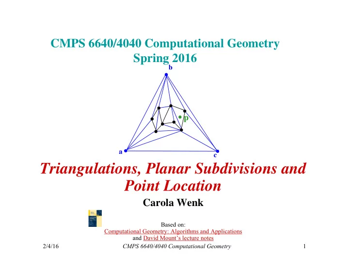
• Given p, if we find a triangle containing p we also know the (label of) the
• riginal subdivision face containing p.

a b c

p

2/4/16 CMPS 6640/4040 Computational Geometry 10

Kirkpatrick’s Hierarchy

• Compute a sequence T0, T1, …, Tk of increasingly coarser triangulations

such that the last one has constant complexity.

• The sequence T0, T1, …, Tk should have the following properties:

– T0 is the input triangulation, Tk is the outer triangle – k  O(log n) – Each triangle in Ti+1 overlaps O(1) triangles in Ti

• How to build such a sequence?

– Need to delete vertices from Ti . – Vertex deletion creates holes, which need to be re-triangulated.

• How do we go from T0 of size O(n) to

Tk of size O(1) in k=O(log n) steps? – In each step, delete a constant fraction

• f vertices from Ti .
• We also need to ensure that each new triangle in Ti+1 overlaps with only

O(1) triangles in Ti .

2/4/16 CMPS 6640/4040 Computational Geometry 11

Vertex Deletion and Independent Sets

When creating Ti+1 from Ti , delete vertices from Ti that have the following properties: – Constant degree: Each vertex v to be deleted has O(1) degree in the graph Ti .

• If v has degree d, the resulting hole can be re-

triangulated with d-2 triangles

• Each new triangle in Ti+1 overlaps at most d original

triangles in Ti

– Independent sets: No two deleted vertices are adjacent.

• Each hole can be re-triangulated independently.

2/4/16 CMPS 6640/4040 Computational Geometry 12

Independent Set Lemma

Lemma: Every planar graph on n vertices contains an independent vertex set of size n/18 in which each vertex has degree at most 8. Such a set can be computed in O(n) time. Use this lemma to construct Kirkpatrick’s hierarchy:

• Start with T0, and select an independent set S of

size n/18 in which each vertex has maximum degree 8. [Never pick the outer triangle vertices a, b, c.]

• Remove vertices of S, and re-triangulate holes.
• The resulting triangulation, T1, has at most 17/18n

vertices.

• Repeat the process to build the hierarchy, until Tk

equals the outer triangle with vertices a, b, c.

• The depth of the hierarchy is k = log18/17 n

a b c

2/4/16 CMPS 6640/4040 Computational Geometry 13

Hierarchy Example

Use this lemma to construct Kirkpatrick’s hierarchy:

• Start with T0, and select an

independent set S of size n/18 in which each vertex has maximum degree 8. [Never pick the outer triangle vertices a, b, c.]

• Remove vertices of S, and re-

triangulate holes.

• The resulting triangulation, T1, has

at most 17/18n vertices.

• Repeat the process to build the

hierarchy, until Tk equals the outer triangle with vertices a, b, c.

• The depth of the hierarchy is

k = log18/17 n

2/4/16 CMPS 6640/4040 Computational Geometry 14

Hierarchy Data Structure

Store the hierarchy as a DAG:

• The root is Tk .
• Nodes in each level correspond to

triangles Ti .

• Each node for a triangle in Ti+1

stores pointers to all triangles of Ti that it overlaps. How to locate point p in the DAG:

• Start at the root. If p is outside of Tk

then p is in exterior face; done.

• Else, set  to be the triangle at the

current level that contains p.

• Check each of the at most 6

triangles of Tk-1 that overlap with , whether they contain p. Update  and descend in the hierarchy until reaching T0 .

• Output  .

p

2/4/16 CMPS 6640/4040 Computational Geometry 15

Analysis

• Query time is O(log n): There are

O(log n) levels and it takes constant time to move between levels.

• Space complexity is O(n):

– Sum up sizes of all triangulations in hierarchy. – Because of Euler’s formula, it suffices to sum up the number of vertices. – Total number of vertices: n + 17/18 n + (17/18)2 n + (17/18)3 n + … ≤ 1/(1-17/18) n = 18 n

• Preprocessing time is O(n log n):

– Triangulating the subdivision takes O(n log n) time. – The time to build the DAG is proportional to its size.

15

p

2/4/16 CMPS 6640/4040 Computational Geometry 16

Independent Set Lemma

Lemma: Every planar graph on n vertices contains an independent vertex set of size n/18 in which each vertex has degree at most 8. Such a set can be computed in O(n) time. Proof: Algorithm to construct independent set:

• Mark all vertices of degree ≥ 9
• While there is an unmarked vertex
• Let v be an unmarked vertex
• Add v to the independent set
• Mark v and all its neighbors
• Can be implemented in O(n) time: Keep list of unmarked

vertices, and store the triangulation in a data structure that allows finding neighbors in O(1) time. v

2/4/16 CMPS 6640/4040 Computational Geometry 17

Independent Set Lemma

Still need to prove existence of large independent set.

• Euler’s formula for a triangulated planar graph on n vertices:

#edges = 3n – 6

• Sum over vertex degrees:

 deg(v) = 2 #edges = 6n – 12 < 6n

• Claim: At least n/2 vertices have degree ≤ 8.

Proof: By contradiction. So, suppose otherwise.  n/2 vertices have degree ≥ 9. The remaining have degree ≥ 3.  The sum of the degrees is ≥ 9 n/2 + 3 n/2 = 6n. Contradiction.

• In the beginning of the algorithm, at least n/2 nodes are unmarked. Each

picked vertex v marks ≤ 8 other vertices, so including itself 9.

• Therefore, the while loop can be repeated at least n/18 times.
• This shows that there is an independent set of size at least n/18 in which

each node has degree ≤ 8.

v

2/4/16 CMPS 6640/4040 Computational Geometry 18

Kirkpatrick’s Hierarchy Summary

• Kirkpatrick’s point location data structure needs O(n log n)

preprocessing time, O(n) space, and has O(log n) query time. It involves rather high constant factors though.

• It can also be used to create a hierarchy of polytopes: The Dobkin-

Kirkpatrick decomposition

2/4/16 CMPS 6640/4040 Computational Geometry 19

Use of Dobkin-Kirkpatrick’s Hierarchy for Polytopes/Polyhedra

Efficiently answer the following types of queries:

• Find an extreme point in a given direction.
• Locate a point on the polytope closest to a query point.
• Compute the intersection of two polytopes ( collision detection)

2/4/16 CMPS 6640/4040 Computational Geometry 20

Extreme Points

Let’s start with 2D: Given a convex polygon (as a list of n vertices in counter-clockwise order around the polygon), how fast can one find a point with maximum y- coordinate? Answer: In O(log n) time using a variant of binary search. What about a convex polytope in 3D? How fast can one find a point on it with maximum z-coordinate? Answer 1: Trivially in O(n) time by checking each vertex. Answer 2: Preprocess the polytope using Dobkin-Kirkpatrick’s hierarchy in O(n log n) time and O(n) space. Then develop an O(log n) time query algorithm.