Transformation based parallel programming Program parallelization - PDF document

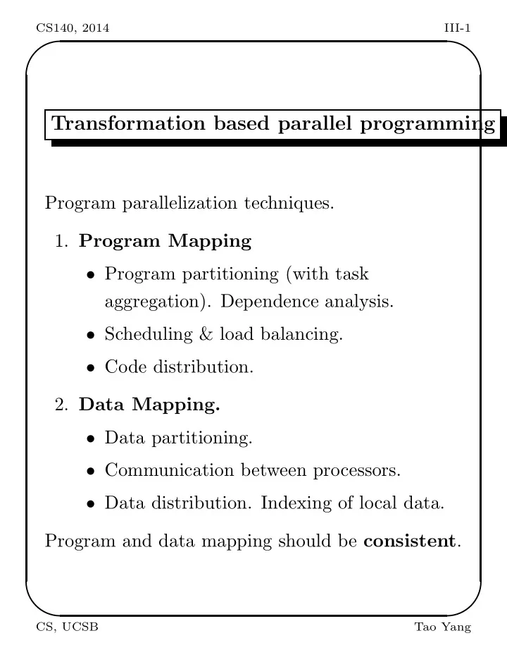
✬ ✩ CS140, 2014 III-1 Transformation based parallel programming Program parallelization techniques. 1. Program Mapping • Program partitioning (with task aggregation). Dependence analysis. • Scheduling & load balancing. • Code distribution. 2. Data Mapping. • Data partitioning. • Communication between processors. • Data distribution. Indexing of local data. Program and data mapping should be consistent . ✫ ✪ CS, UCSB Tao Yang

✬ ✩ CS140, 2014 III-2 An Example Sequential code: x=3 For i = 0 to p-1. y(i)= i*x; Endfor Dependence analysis: x = 3 . . . . (p-1)x 0 x 1 x 2 x Scheduling: Replicate x = 3 (instead of broadcasting). 0 1 2 p-1 x = 3 x = 3 x = 3 x = 3 . . . (p-1)x 0 x 1x 2 x ✫ ✪ CS, UCSB Tao Yang

✬ ✩ CS140, 2014 III-3 SPMD Code: int x,y,i; x = 3; i = mynode(); y = i * x; Data and program distribution : Sequential Parallel (one node) Data Array y [0 , 1 , . . . , p − 1] = ⇒ Element y program = ⇒ y = i ∗ x For i=0 to p-1 y(i) = i*x ✫ ✪ CS, UCSB Tao Yang

✬ ✩ CS140, 2014 III-4 Dependence Analysis • For each task, define the input and output sets. INPUT OUTPUT Task Example : S : A = C + B IN(S) = { C,B } OUT(S) = { A } . • Given a program with two tasks: S 1 , S 2 . If changing execution order of S 1 and S 2 affects the result. = ⇒ S 2 depends on S 1 . • Type of dependence: 1. Flow dependence (true data dependence). 2. Output dependence. Anti dependence. – Useful in a shared memory machine. 3. Control dependence ( e.g. if A then B). ✫ ✪ CS, UCSB Tao Yang

✬ ✩ CS140, 2014 III-5 • Flow Dependence: OUT( S 1 ) ∩ IN( S 2 ) � = φ S 1 : A = x + B S 2 : C = A + 3 S2 is dataflow-dependent on S1. • Output Dependence: OUT( S 1 ) ∩ OUT( S 2 ) � = φ . S 1 : A = 3 S 2 : A = x S2 is output-dependent on S1. • Anti Dependence: IN( S 1 ) ∩ OUT( S 2 ) � = φ . S 1 : B = A + 3 S 2 : A = x + 5 S2 is anti-dependent on S1. ✫ ✪ CS, UCSB Tao Yang

✬ ✩ CS140, 2014 III-6 Coarse-grain dependence graph. Tasks operate on data items of large sizes and perform a large chunk of computations. Assume each function below only reads input Ex : S 1 : A = f(X,B) parameters. S 2 : C = g(A) S 3 : A = h(A,C) S 1 Flow Flow Output S 2 Flow Anti S 3 ✫ ✪ CS, UCSB Tao Yang

✬ ✩ CS140, 2014 III-7 Delete redundant dependence edges The deletion should not affect the correctness. An anti or output dependence edge can be deleted if it is subsumed by another dependence path. S 1 Flow Flow S 2 Flow S 3 ✫ ✪ CS, UCSB Tao Yang

✬ ✩ CS140, 2014 III-8 Loop Parallelism Iteration space – all iterations of a loop and data dependence between iteration statements. 1 D Loop: For i = 1 to n S : a = b + c i i i i . . . S 2 S 3 S n S 1 For i = 1 to n S : a = a - 1 i i i-1 . . . S 2 S n S 1 2 D Loop: j S S S 11 12 13 For i = 1 to n For j = 1 to n S S S 21 23 22 S : x = x +1 ij ij i-1,j S S S i 31 32 33 ✫ ✪ CS, UCSB Tao Yang

✬ ✩ CS140, 2014 III-9 Program Partitioning Purpose: • Increase task granularity (task grain size). • Reduce unnecessary communication. • Ease the mapping of a large number of tasks to a small number of processors. Actions: Group several tasks together as one task. Loop partitioning techniques: • Loop blocking/unrolling. • Interior loop blocking. • Loop interchange. ✫ ✪ CS, UCSB Tao Yang

✬ ✩ CS140, 2014 III-10 Loop blocking/unrolling Given: For i=1 to 2n S i : a i = b i + c i Block this loop by a factor of 2 or unroll this loop by a factor of 2. . . . S S 1 S 2 S 3 S 4 S 2n 2n-1 . . . n 2 1 After transformation: = ⇒ For i = 1 n to S 2 i − 1 , S 2 i do ✫ ✪ CS, UCSB Tao Yang

✬ ✩ CS140, 2014 III-11 General 1D Loop Blocking Given: For i = 1 to r*p S i : a(i) = b(i)+c(i) Block this loop by a factor of r : For j = 0 to p-1 For i = r*j+1 to r*j+r a(i) = b(i)+c(i) SPMD code on p nodes . me=mynode(); For i = r*me+1 to r*me+r a(i) = b(i)+c(i) ✫ ✪ CS, UCSB Tao Yang

✬ ✩ CS140, 2014 III-12 Interior Loop Partitioning Block the interior loop and make it one task. Example: i = 1 4 For to j = 1 to 4 For x i,j = x i,j − 1 + 1 After blocking: i = 1 4 For to j = 1 to 4 For x i,j = x i,j − 1 + 1 j i i The above example preserves the parallelism. ✫ ✪ CS, UCSB Tao Yang

✬ ✩ CS140, 2014 III-13 Partitioning may reduce parallelism i = 1 4 For to j = 1 to 4 For x i,j = x i − 1 ,j + 1 j i i No inter-task parallelism! ✫ ✪ CS, UCSB Tao Yang

✬ ✩ CS140, 2014 III-14 Loop Interchange Definition: A program transformation that changes the execution order of a loop program. Actions: Swap the loop control statements. Example: i = 1 4 For to j = 1 to 4 For x i,j = x i − 1 ,j + 1 After loop interchange: j = 1 4 For to i = 1 to 4 For x i,j = x i − 1 ,j + 1 ✫ ✪ CS, UCSB Tao Yang

✬ ✩ CS140, 2014 III-15 Why loop interchange? Usage: Help loop partitioning for better performance. Example . Interior loop blocking after interchange . j = 1 4 For to i = 1 to 4 For x ij = x i − 1 j + 1 j i ✫ ✪ CS, UCSB Tao Yang

✬ ✩ CS140, 2014 III-16 Execution order after loop interchange Loop interchange alters the execution order. j S12 S13 S11 For i = 1 to 3 For j= 1 to 3 S23 S22 S21 S i,j : S32 S33 S31 i Execution order j S12 S13 S11 For j= 1 to 3 For i = 1 to 3 S23 S22 S21 S i,j : S32 S33 S31 i ✫ ✪ CS, UCSB Tao Yang

✬ ✩ CS140, 2014 III-17 Not every loop interchange is legal in the sequential code Loop interchange is not legal if the new execution order violates data dependence. For i = 1 to 3 j For j= 1 to 3 S12 S13 S11 Execution order S i,j : X(i,j)=X(i−1,j+1)+1 S23 S22 S21 Dependence Legal? S32 S33 S31 i j For j= 1 to 3 For i = 1 to 3 S12 S13 S11 S i,j : X(i,j)=X(i−1,j+1)+1 S23 S22 S21 S32 S33 S31 i Parallel code execution needs to make sure data dependence is satisfied when loop interchange is ✫ ✪ used. CS, UCSB Tao Yang

✬ ✩ CS140, 2014 III-18 Interchanging triangular loops = ⇒ For j=2 to 10 For i=1 to 10 For j=i+1 to 10 For i=1 to j-1 2 10 j 2 10 j 1 1 i i j=i+1 ✫ ✪ CS, UCSB Tao Yang

✬ ✩ CS140, 2014 III-19 Transformation for loop interchange How to derive the new bounds for i and j loops? • Step 1: List all inequalities regarding i and j from the original code. i ≤ 10 , i ≥ 1 , j ≤ 10 , j ≥ i + 1 . • Step 2: Derive bounds for loop j . – Extract all inequalities regarding the upper bound of j . j ≤ 10 . The upper bound is 10. – Extract all inequalities regarding the lower bound of j . j ≥ i + 1 . The lower bound is 2 since i could be as low as 1. • Step 3: Derive bounds for loop i when j ✫ ✪ CS, UCSB Tao Yang

✬ ✩ CS140, 2014 III-20 value is fixed (now loop i is an inner loop). – Extract all inequalities regarding the upper bound of i . i ≤ 10 , i ≤ j − 1 . The upper bound is min(10 , j − 1). – Extract all inequalities regarding the lower bound of i . i ≥ 1 . The lower bound is 1. ✫ ✪ CS, UCSB Tao Yang

✬ ✩ CS140, 2014 III-21 Data Partitioning and Distribution Data structure is divided into data units and assigned to processor local memories. Why? • Not enough space for replication for solving large problems. • Partition data among processors so that data accessing is localized for tasks. Ex : y = A n × n · x proc 0 n/p proc 1 n/p . proc 2 x . . n/p Distribute array A among p nodes. But replicate x to all processors. ✫ ✪ CS, UCSB Tao Yang

✬ ✩ CS140, 2014 III-22 Corresponding Task Mapping: ( r = n/p ) P 0 P 1 · · · A 1 x A r +1 x A 2 x A r +2 x . . . . . . A r x A 2 r x ✫ ✪ CS, UCSB Tao Yang

✬ ✩ CS140, 2014 III-23 1D Data Mapping Methods 1D array − → 1D processors . • Assume that data items are counted from 0 , 1 , · · · n − 1. • Processors are numbered from 0 to p − 1. Mapping methods: Let r = ⌈ n p ⌉ . • 1D Block r p 0 1 2 3 Data = ⇒ Proc ⌊ i i r ⌋ ✫ ✪ CS, UCSB Tao Yang

✬ ✩ CS140, 2014 III-24 • 1D Cyclic 0 1 2 3 0 1 2 3 0 1 2 3 0 1 2 3 p Data = ⇒ Proc i i mod p • 1D Block Cyclic. First the array is divided into a set of units using block partitioning (block size b ). Then these units are mapped in a cyclic manner to p processors. r r r r r r r r p 0 1 2 3 0 1 2 3 Data = ⇒ Proc ⌊ i i b ⌋ mod p ✫ ✪ CS, UCSB Tao Yang

✬ ✩ CS140, 2014 III-25 2D array − → 1D processors 2D data space is partitioned into a 1D space. Then partitioned data items are counted from 0 , 1 , · · · n − 1. Processors are numbered from 0 to p − 1. Methods: • Column-wise block. (call it (*,block)) Data ( i, j ) ⇒ Proc ⌊ j r ⌋ Proc 1 3 0 2 Proc 0 Proc 1 Proc 2 Proc 3 • Row-wise block. (call it (block,*)) Data ( i, j ) ⇒ Proc ⌊ i r ⌋ ✫ ✪ CS, UCSB Tao Yang

✬ ✩ CS140, 2014 III-26 • Row cyclic. (cyclic,*) Data ( i, j ) ⇒ Proc i mod p . • Others: Column cyclic. Column block cyclic. Row block cyclic · · · . ✫ ✪ CS, UCSB Tao Yang