Towards Unbiased BFS Sampling Maciej Kurant Athina Markopoulou - - PDF document

▶

Sep 06, 2023 425 likes •587 views

Towards Unbiased BFS Sampling Maciej Kurant Athina Markopoulou Patrick Thiran EECS Dept EECS Dept School of Computer & Comm. Sciences University of California, Irvine University of California, Irvine EPFL, Lausanne, Switzerland

SLIDE 1

arXiv:1102.4599v1 [cs.SI] 22 Feb 2011

Towards Unbiased BFS Sampling

Maciej Kurant

EECS Dept University of California, Irvine maciej.kurant@gmail.com

Athina Markopoulou

EECS Dept University of California, Irvine athina@uci.edu

Patrick Thiran

School of Computer & Comm. Sciences EPFL, Lausanne, Switzerland patrick.thiran@epfl.ch

Abstract—Breadth First Search (BFS) is a widely used approach for sampling large unknown Internet topologies. Its main advantage over random walks and other exploration techniques is that a BFS sample is a plausible graph on its own, and therefore we can study its topological characteristics. However, it has been empirically observed that incomplete BFS is biased toward high- degree nodes, which may strongly affect the measurements. In this paper, we first analytically quantify the degree bias

f BFS sampling. In particular, we calculate the node degree

distribution expected to be observed by BFS as a function of the fraction f of covered nodes, in a random graph RG(pk) with an arbitrary degree distribution pk. We also show that, for RG(pk), all commonly used graph traversal techniques (BFS, DFS, Forest Fire, Snowball Sampling, RDS) suffer from exactly the same bias. Next, based on our theoretical analysis, we propose a practical BFS-bias correction procedure. It takes as input a collected BFS sample together with its fraction f. Even though RG(pk) does not capture many graph properties common in real-life graphs (such as assortativity), our RG(pk)-based correction technique performs well on a broad range of Internet topologies and on two large BFS samples of Facebook and Orkut networks. Finally, we consider and evaluate a family of alternative correction procedures, and demonstrate that, although they are unbiased for an arbitrary topology, their large variance makes them far less effective than the RG(pk)-based technique. Index Terms—BFS, Breadth First Search, graph sampling, estimation, bias correction, Internet topologies, Online Social Networks.

I. INTRODUCTION

A large body of work in the networking community focuses

n Internet topology measurements at various levels, including

the IP or AS connectivity, the Web (WWW), peer-to-peer (P2P) and online social networks (OSN). The size of these networks and other restrictions make measuring the entire graph impossible. For example, learning only the topology of Facebook social graph would require downloading more than 250T B of HTML data [2,3], which is most likely impractical. Instead, researchers typically collect and study a small but representative sample of the underlying graph. In this paper, we are particularly interested in sampling networks that naturally allow to explore the neighbors of a given node (which is the case in WWW, P2P and OSN). A number of graph exploration techniques use this basic

peration for sampling. They can be roughly classified in two

categories: (i) random walks, and (ii) graph traversals. In the first category, random walks, nodes can be revisited. This category includes the classic Random Walk (RW) [4] and

This paper is a revised and extended version of [1].

qk expected observed

average node degree

k2 k

f fraction of sampled nodes 1

Random Walk (RW) Graph traversal techniques:

BFS
DFS
Forest Fire
Snowball / RDS

Metropolis-Hastings Random Walk (MHRW)

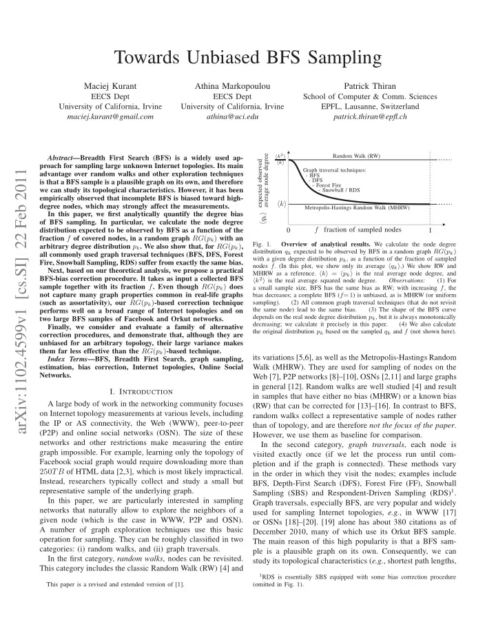
Fig. 1.

Overview of analytical results. We calculate the node degree distribution qk expected to be observed by BFS in a random graph RG(pk) with a given degree distribution pk, as a function of the fraction of sampled nodes f. (In this plot, we show only its average qk.) We show RW and MHRW as a reference. k = pk is the real average node degree, and k2 is the real average squared node degree. Observations: (1) For a small sample size, BFS has the same bias as RW; with increasing f, the bias decreases; a complete BFS (f=1) is unbiased, as is MHRW (or uniform sampling). (2) All common graph traversal techniques (that do not revisit the same node) lead to the same bias. (3) The shape of the BFS curve depends on the real node degree distribution pk, but it is always monotonically decreasing; we calculate it precisely in this paper. (4) We also calculate the original distribution pk based on the sampled qk and f (not shown here).

its variations [5,6], as well as the Metropolis-Hastings Random Walk (MHRW). They are used for sampling of nodes on the Web [7], P2P networks [8]–[10], OSNs [2,11] and large graphs in general [12]. Random walks are well studied [4] and result in samples that have either no bias (MHRW) or a known bias (RW) that can be corrected for [13]–[16]. In contrast to BFS, random walks collect a representative sample of nodes rather than of topology, and are therefore not the focus of the paper. However, we use them as baseline for comparison. In the second category, graph traversals, each node is visited exactly once (if we let the process run until com- pletion and if the graph is connected). These methods vary in the order in which they visit the nodes; examples include BFS, Depth-First Search (DFS), Forest Fire (FF), Snowball Sampling (SBS) and Respondent-Driven Sampling (RDS)1. Graph traversals, especially BFS, are very popular and widely used for sampling Internet topologies, e.g., in WWW [17]

r OSNs [18]–[20]. [19] alone has about 380 citations as of

December 2010, many of which use its Orkut BFS sample. The main reason of this high popularity is that a BFS sample is a plausible graph on its own. Consequently, we can study its topological characteristics (e.g., shortest path lengths,

1RDS is essentially SBS equipped with some bias correction procedure

(omitted in Fig. 1).

SLIDE 2

clustering coefficients, community structure), which is a big advantage of BFS over random walks. Of course, this approach is correct only if the BFS sample is representative of the entire

graph. At first sight it seems true, e.g., a BFS sample of a

lattice is a (smaller) lattice. Unfortunately, this intuition often fails. It was observed empirically that BFS introduces a bias towards high-degree nodes [17,21]–[23]. We also confirmed this fact in a recent measurement of Facebook [2,3], where our BFS crawler found the average node degree 324, while the real value is only 94. This means that the average node degree is overestimated by BFS by about 250%! This has a striking effect not only on the node property statistics, but also on the topological metrics. Despite the popularity of BFS on the one hand, and its bias on the other hand, we still know relatively little about the statistical properties of node sequences returned by BFS. The formal analysis is challenging because BFS, similarly to every sampling without replacement, introduces complex dependencies between the sampled nodes difficult to deal with mathematically. Contributions. Our work is a step towards understanding the statistical characteristics of BFS samples and correcting for their biases, with the following main contributions. First, we focus on a random graph RG(pk) with a given (and arbitrary) degree distribution pk. We calculate precisely the node degree distribution qk expected to be observed by BFS as a function of the fraction f of sampled nodes. We illustrate this and related results in Fig. 1. To the best of our knowledge, this is the first analytical result describing the bias

f BFS sampling.

Second, based on our theoretical analysis, we propose a practical BFS-bias correction procedure. It takes as input a collected BFS sample together with the fraction f of covered nodes, and estimates the mean of an arbitrary function x(v) defined on graph nodes. Even though RG(pk) misses many graph properties common in real-life graphs (such as assortativity), our RG(pk)-based correction technique performs well

n a broad range of Internet topologies, and on two large BFS

samples of Facebook and Orkut networks. We make its ready- to-use python implementation publicly available at [24]. Third, we complement the above findings by proposing a family of alternative correction procedures that are unbiased for any arbitrary topology. Although seemingly attractive, they are characterized by large variance, which makes them far less effective than the RG(pk)-based correction technique.

Scope. Our theoretical results hold strictly for the random

graph model RG(pk). (However, we show that they apply relatively well to a broad range of real-life topologies.) We also restrict our attention to static graphs with self-declared un- weighted social links; dynamically varying graphs [8,10,25]– [30] and interaction graphs [31]–[33] are out of the scope of this paper. Finally, our RG(pk)-based bias-correction procedure is designed for local graph properties, such as node statistics. Our analytical results can potentially help the estimation of non- local graph properties (such as graph diameter), which is our main direction for the future.

Outline. The outline of the paper is as follows. Section II

discusses related work. Section III presents BFS and other graph traversal algorithms under study. We also briefly describe random walks that are used as baseline for comparison throughout the paper. Section IV presents the random graph RG(pk) model used in this paper. Section V analyzes the degree bias of BFS. Section VI shows how to correct for this bias. Section VII evaluates our results in simulations and by sampling real world networks. Section VIII introduces and evaluates alternative BFS-bias correction techniques. Sec- tion IX gives some practical sampling recommendations, and Section X concludes the paper.

II. RELATED WORK

BFS used in practice. BFS is widely used today for ex- ploring large networks, such as OSNs. In [18], Ahn et al. used BFS to sample Orkut and MySpace. In [19] and [27], Mislove et al. used BFS to crawl the social graph in four popular OSNs: Flickr, LiveJournal, Orkut, and YouTube. [19] alone has about 380 citations as of December 2010, many of which use its highly biased Orkut BFS sample. In [20], Wilson et al. measured the social graph and the user interaction graph

f Facebook using several BFSs, each BFS constrained in one
f the largest 22 regional Facebook networks. In our recent

work [2,3], we have also crawled Facebook using various sampling techniques, including BFS, RW and MHRW. BFS bias. It has been empirically observed that incomplete BFS and its variants introduce bias towards high-degree nodes [17] [21]–[23]. We confirmed this in Facebook [2,3], which, in fact, inspired and motivated this paper. Analogous bias has been observed in the field of social science, for sampling techniques closely related to BFS, i.e., Snowball Sampling and RDS [15,34,35] (see Section III-B4). Analyzing BFS. To the best of our knowledge, the sampling bias of BFS has not been analyzed so far. [36] and [37] are the closest related papers to our methodology. The original paper by Kim [36] analyzes the size of the largest connected component in classic Erd¨

s-R´

enyi random graph by essentially applying the configuration model with node degrees chosen from a Poisson distribution. To match the stubs (or “clones” in [36]) uniformly at random in a tractable way, Kim proposes a “cut-off line” algorithm. He first assigns each stub a random index from [0, np], and next progressively scans this interval. Achlioptas et al. used this powerful idea in [37] to study the bias of traceroute sampling in random graphs with a given degree distribution. The basic operation in [37] is traceroute (i.e., “discover a path”) and is performed from a single node to all other nodes in the graph. The union of the observed paths forms a “BFS-tree”, which includes all nodes but misses some edges (e.g., those between nodes at the same depth in the tree). In contrast, the basic operation in the traversal methods presented in our paper is to discover all neighbors of a node, and it is applied to all nodes in increasing distance from the origin. Another important difference is that [37] studies a

SLIDE 3

completed BFS-tree, whereas we study the sampling process when it has visited only a fraction f < 1 of nodes. Indeed, a completed BFS (f=1) is trivial in our case: it has no bias, as all nodes are covered. In the field of social science, a significant effort was put to correct for the bias of BFS’s close cousin - Snowball Sampling (SBS) [34]. SBS together with a bias correction procedure is called Respondent-Driven Sampling (RDS) [35]. The currently used correction technique [15,16] assumes that nodes can be revisited, which essentially approximates SBS by Random Walk (see Section VI-A1). In this paper, we formally show that this approximation is valid if the fraction f of sampled nodes is relatively small. However, as [38] points out, the current RDS methodology is systematically biased for larger f. Consequently, [39] proposed an SBS bias correction method based on the random graph RG(pk). This is essentially the same basic starting idea as used in our original paper published independently [1]. However, the two papers fundamentally differ in the final solution: [39] proposes a simulation-aided approach, whereas we solve the problem analytically. Another recent and related paper is [40]. The authors propose and evaluate a heuristic approach to correct the degree bias in the ith generation of SBS, based on the values measured in the generation i − 1. In practice, this generation-based scheme may be challenging to implement, because the number of nodes per generation may grow close to exponential with i. Consequently, we are likely to face a situation where collecting the next generation is prohibitively expensive, while the current generation has much fewer nodes than our sampling capabilities allow for. Probability Proportional to Size Without Replacement (PPSWOR). At a closer look, our RG(pk)-based approach reduces BFS (and other graph traversals) to a classic sampling design called Probability Proportional to Size Without Replacement (PPSWOR) [41]–[48]. Unfortunately, to the best

f our knowledge, none of the existing results is directly

applicable to our problem. This is because, speaking in the terms used later in this paper, the available results either (i) require the knowledge of qk(f) (expected, not sampled) as an input, (ii) propose how to calculate qk(f) for the first two nodes only, or (iii) calculate qk(f) as an average of many simulated traversals of the known graph (in contrast, we only have one run on unknown graph) [48]. In fact, this work can be naturally extended to address the problems with PPSWOR. Previous version of this paper. This work is a revised and extended version of our recent conference paper [1]. The main changes are: (i) a successful application of our RG(pk)-based correction procedure to a wide range of large-scale real-life Internet topologies (Table II, Fig. 5, Fig. 6(d), Section VII-B), (ii) bias correction procedures for arbitrary node properties (Section VI), (iii) a complementary BFS-bias correction technique (Section VIII), and (iv) a publicly available ready-to-use python implementation of our approach. Finally, we would like to stress that our two other JSAC submissions [3,49] focus on sampling techniques based on random walks, which differ in fundamental aspects (sampling with replacement vs without, sampling of nodes vs of topol-

gy) from the BFS sampling addressed here.
III. GRAPH EXPLORATION TECHNIQUES

Let G = (V, E) be a connected graph with the set of vertices V , and a set of undirected edges E. Initially, G is unknown, except for one (or some limited number of) seed node(s). When sampling through graph exploration, we begin at the seed node, and we recursively visit (one, some or all) its

neighbors. We distinguish two main categories of exploration

techniques: random walks and graph traversals.

A. Random walks (baseline)

Random walks allow revisiting the same node many times. We consider2 the following classic examples: 1) Random Walk (RW): In this classic sampling technique [4], we start at some seed node. At every iteration, the next-hop node v is chosen uniformly at random among the neighbors of the current node u. It is easy to see that RW introduces a linear bias towards nodes of high degree [4]. 2) Metropolis Hastings Random Walk (MHRW): In this technique, as in RW, the next-hop node w is chosen uniformly at random among the neighbors of the current node u. How- ever, with a probability that depends on the degrees of w and u, MHRW performs a self-loop instead of moving to w. More specifically, the probability P MH

u,w of moving from u to w is as

follows [50]: P

u,w =

  

1 ku · min(1, ku kw )

if w is a neighbor of u, 1 −

y=u P MH u,y

if w = u,

therwise,

(1) where kv is the degree of node v. Essentially, MHRW reduces the transitions to high-degree nodes and thus eliminates the degree bias of RW. This property of MHRW was recently exploited in various network sampling contexts [2,8,10,11].

B. Graph traversals

In contrast, graph traversals never revisits the same node. At the end of the process, and assuming that the graph is connected, all nodes are visited. However, when using graph traversals for sampling, we terminate after having collected a fraction f < 1 (usually f ≪ 1) of graph nodes. 1) Breadth First Search (BFS): BFS is a classic graph traversal algorithm that starts from the seed and progressively explores all neighbors. At each new iteration the earliest explored but not-yet-visited node is selected next. Consequently, BFS discovers first the nodes closest to the seed. 2) Depth First Search (DFS): This technique is similar to BFS, except that at each iteration we select the latest explored but not-yet-visited node. As a result, DFS explores first the nodes that are faraway (in the number of hops) from the seed.

2We include random walks only as a useful baseline for comparison with

graph traversals (e.g., BFS). The analysis of random walks does not count as a contribution of this paper.

SLIDE 4

G = (V, E) graph G with nodes V and edges E kv degree of node v pk =

1 |V |

v∈V 1kv=k

degree distribution in G k = pk =

k k pk

average node degree in G qk expected sampled degree distribution qk =

k k qk

expected sampled average node degree

sampled degree distribution

estimated original degree distribution in G f fraction of nodes covered by the sample TABLE I NOTATION SUMMARY.

3) Forest Fire (FF): FF is a randomized version of BFS, where for every neighbor v of the current node, we flip a coin, with probability of success p, to decide if we explore v. FF reduces to BFS for p= 1. It is possible that this process dies

ut before it covers all nodes. In this case, in order to make FF

comparable with other techniques, we revive the process from a random node already in the sample. Forest Fire is inspired by the graph growing model of the same name proposed in [51] and is used as a graph sampling technique in [12]. 4) Snowball Sampling (SBS) and Respondent-Driven Sam- pling (RDS): According to a classic definition by Good- man [34], an n-name Snowball Sampling is similar to BFS, but at every node v, not all kv, but exactly n neighbors are chosen randomly out of all kv neighbors of v. These n neighbors are scheduled to visit, but only if they have not been visited before. Respondent-Driven Sampling (RDS) [15,16,35] adopts SBS to penetrate hidden populations (such as that of drug addicts) in social surveys. In Section II, we comment on current techniques to correct for SBS/RDS bias towards nodes of higher degree.

IV. GRAPH MODEL RG(pk)

A basic, yet very important property of every graph is its node degree distribution pk, i.e., the fraction of nodes with degree equal to k, for all k ≥ 0.3 Depending on the network, the degree distribution can vary, ranging from constant-degree (in regular graphs), a distribution concentrated around the average value (e.g., in Erd¨

s-R´

enyi random graphs or in well- balanced P2P networks), to heavily right-skewed distributions with k covering several decades (as this is the case in WWW, unstructured P2P, Internet at the IP and Autonomous System level, OSNs). We handle all these cases by assuming that we are given any fixed node degree distribution pk. Other than that, the graph G is drawn uniformly at random from the set

f all graphs with degree distribution pk. We denote this model

by RG(pk). Because RG(pk) mimics an arbitrary node degree distribution pk, it can be considered a “first-order approximation” of real-life graphs. Of course, there are many graph properties

ther than pk that are not captured by RG(pk). However, we

show later that, with respect to the BFS sampling bias, RG(pk) approximates the real Internet topologies surprisingly well. We use a classic technique to generate RG(pk), called the configuration model [52]: each node v is given kv “stubs”

3As we define pk as a ‘fraction’, not the ‘probability’, pk determines the

degree sequence in the graph, and vice versa.

r “edges-to-be”. Next, all these

v∈V kv = 2|E| stubs are

randomly matched in pairs, until all stubs are exhausted (and |E| edges are created). In Fig. 2 (ignore the rectangular interval [0,1] for now), we present four nodes with their stubs (left) and an example of their random matching (right).

V. ANALYZING THE NODE DEGREE BIAS

In this section, we study the node degree bias observed when the graph exploration techniques of Section III are run

n the random graph RG(pk) of Section IV. In particular,

we are interested in the node degree distribution qk expected to be observed in the raw sample. Typically, the observed distribution is different from the original one, qk = pk, with higher average value qk > pk (i.e., average sampled and

bserved node degree, respectively). Below, we derive qk as

a function of pk and, in the case of BFS, of the fraction of sampled nodes f.

A. Random walks (baseline)

We begin by summarizing the relevant results known for walks, in particular for RW and MHRW. They will serve as a reference point for our main analysis of graph traversals below. 1) Random Walk (RW): Random walks have been widely studied; see [4] for an excellent survey. In any given connected and aperiodic graph, the probability of being at a particular node v converges at equilibrium to the stationary distribution πRW

kv 2|E|. Therefore, the expected observed degree

distribution qRW

k is

v · 1{kv=k} =

k 2|E| pk |V | = k pk k , (2) where k is the average node degree in G. Eq.(2) is essentially similar to calculation in [13]–[16]. As this holds for any fixed (and connected and aperiodic) graph, it is also true for all connected graphs generated by the configuration model. Consequently, the expected observed average node degree is q

k =

k q

k k2 pk

k = k2 k , (3) where k2 is the average squared node degree in G. We show this value k2

k in Fig. 1.

2) Metropolis Hastings Random Walk (MHRW): It is easy to show that the transition matrix P MH

u,w shown in Eq.(1)

leads to a uniform stationary distribution πMH

v = 1 |V | [50], and

consequently: q

= pk (4) q

k q

k pk = k. (5) In Fig. 1, we show that MHRW estimates the true mean.

SLIDE 5

B. Graph traversals (Main Result)

In both RW and MHRW the nodes can be revisited. So the state of the system at iteration i + 1 depends only on iteration i, which makes it possible to analyze with Markov Chain techniques. In contrast, graph traversals do not allow for node revisits, which introduces crucial dependencies between all the iterations and significantly complicates the analysis. To handle these dependencies, we adopt an elegant technique recently introduced in [36] (to study the size of the largest connected component) and extended in [37] (to study the bias

f traceroute sampling). However, our work differs in many

aspects from both [36] and [37], on which we comment in detail in the related work Section II. 1) Exploration without replacement at the stub level: We begin by defining Algorithm 1 (below) - a general graph traversal technique that collects a sequence of nodes S, without

replacements. To be compatible with the configuration model

(see Section IV), we are interested in the process at the stub level, where we consider one stub at a time, rather than one node at a time. An integral part of the algorithm is a queue Q that keeps the discovered, but still not-yet-followed stubs. First, we enqueue on Q all the stubs of some initial node v1, and by setting S ←[v1]. Next, at every iteration, we dequeue

ne stub from Q, call it a, and follow it to discover its partner-

stub b, and b’s owner v(b). If node v(b) is not yet discovered, i.e., if v(b) / ∈ S, then we append v(b) to S and we enqueue

n Q all other stubs of v(b).

Algorithm 1 Stub-Level Graph Traversal

1: S ← [v1] and Q ← [all stubs of v1] 2: while Q is nonempty do 3:

Dequeue a from Q

Discover a’s partner b

if v(b) / ∈ S then

Append v(b) to S

Enqueue on Q all stubs of v(b) except b

else

Remove b from Q

10:

end if

11: end while

Depending on the scheduling discipline for the elements in Q (line 3), Algorithm 1 implements BFS (for a first-in first

ut scheduling), DFS (last-in first-out) or Forest Fire (first-

in first-out with randomized stub losses). Line 9 guarantees that the algorithm never tracebacks the edges, i.e., that stub a dequeued from Q in line 3 never belongs to an edge that has already been traversed in the opposite direction. 2) Discovery on-the-fly: In line 4 of Algorithm 1, we follow stub a to discover its partner b. In a fixed graph G, this step is deterministic. In the configuration model RG(pk), a fixed graph G is obtained by matching all the stubs uniformly at

random. Next, we can sample this fixed graph and average the

result over the space of all the random graphs RG(pk) that have just been constructed. Unfortunately, this space grows exponentially with the number of nodes |V |, making the problem untractable. Therefore, we adopt an alternative construction of G - by iteratively selecting b on-the-fly (i.e., every time line 4 is executed), uniformly at random from all still unmatched stubs. By the principle of deferred decisions [53], these two approaches are equivalent. With the help of the on-the-fly approach, we are able to write down the equations we need. Indeed, let us denote by Xi ∈ V the ith selected node, and let P(X1 = u) be the probability that node u ∈ V is chosen as a starting node. It is easy to show that with z=2|E| we have

P(X2=v) =

kv z−ku · P(X1=u) (6) P(X3=w) =

v=w
u=w,v

kw z−kv−ku · kv z−ku · P(X1=u), (7)

and so on. Theoretically, these equations allow us to calculate the expected node degree at any iteration, and thus the degree bias of BFS. 3) Breaking the dependencies: There is still one problem with the equations above. Due to the increasing number of nested sums, the results can be calculated in practice for a first few iterations only. This is because we select stub b uniformly and independently at random from all the unmatched stubs. So the stub selected at iteration i depends on the stubs selected at iterations 1 . . . i−1, which results in the nested sums. We remedy this problem by implementing the on-the-fly approach as follows. First, we assign each stub a real-valued index t drawn uniformly at random from the interval [0, 1]. Then, every time we process line 4, we pick b as the unmatched stub with the smallest index. We can interpret this as a continuous- time process, where we determine progressively the partners

f stubs dequeued from Q, by scanning the interval from

time t= 0 to t= 1 in a search of unmatched stubs. Because the indices chosen by the stubs are independent from each

ther, the above trick breaks the dependence between the stubs,

which is crucial for making this approach tractable. In Fig. 2, we present an example execution of Algorithm 1, where line 4 is implemented as described above. 4) Expected sampled degree distribution qBFS

k : Now we are

ready to derive the expected observed degree distribution qk. Recall that all the stub indices are chosen independently and uniformly from [0, 1]. A vertex v with degree k is not sampled yet at time t if the indices of all its k stubs are larger than t, which happens with probability (1−t)k. So the probability that v is sampled before time t is 1−(1−t)k. Therefore, the expected fraction of vertices of degree k sampled before t is fk(t) = pk(1−(1−t)k). (8) By normalizing Eq.(8), we obtain the expected observed (i.e., sampled) degree distribution at time t: q

BFS

k (t) =

fk(t)

l fl(t) =

pk(1 − (1−t)k)

l pl(1 − (1−t)l).

(9)

SLIDE 6

3 4 3 1 1 1 1 2 2 2 1 1 1 3 4 3 1

time t (index) time t (index) current time t

v1 v1 v1 v2 v2 v2 v3 v3 v3 v4 v4 v4

Fig. 2.

An illustration of the stub-level, on-the-fly graph exploration without replacements. In this particular example, we show an execution of BFS starting at node v1. Left: Initially, each node v has kv stubs, where kv is a given target degree of v. Each of these stubs is assigned a real-valued number drawn uniformly at random from the interval [0, 1] shown below the graph. Next, we follow Algorithm 1 with a starting node v1. The numbers next to the stubs

f every node v indicate the order in which these stubs are enqueued on Q.

Center: The state of the system at time t. All stubs in [0, t] have already been matched (the indices of matched stubs are set in plain line). All unmatched stubs are distributed uniformly at random on (t, 1]. This interval can contain also some (here two) already matched stubs. Right: The final result is a realization of a random graph G with a given node degree sequence (i.e., of the configuration model). G may contain self-loops and multiedges.

Unfortunately, it is difficult to interpret qBFS

k (t) directly, be-

cause t is proportional neither to the number of matched edges nor to the number of discovered nodes. Recall that our primary goal is to express qBFS

as a function of fraction f of covered

nodes. We achieve this by calculating f(t) - the expected

fraction of nodes, of any degree, visited before time t f(t) =

fk(t) = 1 −

pk(1−t)k . (10) Because pk ≥ 0, and pk > 0 for at least one k > 0, the term

k pk(1−t)k is continuous and strictly decreasing from 1 to

0 with t growing from 0 to 1. Thus, for f ∈ [0, 1] there exists a well defined t=t(f) that satisfies Eq.(10), i.e., the inverse of f(t). Although we cannot compute t(f) analytically (except in some special cases such as for k ≤ 4), it is straightforward to find it numerically. Now, we can rewrite Eq. (9) as q

BFS

k (f) =

pk(1 − (1−t(f))k)

l pl(1 − (1−t(f))l),

(11) which is the expected observed degree distribution after covering fraction f of nodes of graph G. Consequently, the expected

bserved average degree is

BFS

k (f) =

k · q

BFS

k (f).

(12) In other words, Eq.(11) and Eq.(12) describe the bias of BFS sampling under RG(pk), which was our first goal in this paper. Below, we further analyze these equations to get more insights in the nature of BFS bias. 5) Equivalence of traversal techniques under RW(pk): An interesting observation is that, under the random graph model RW(pk), all common traversal techniques (BFS, DFS, FF, SBS, etc) are subject to exactly the same bias. The explanation is that the sampled node sequence S is fully determined by the choice of stub indices on [0, 1], independently of the way we manage the elements in Q. 6) Equivalence of traversals to weighted sampling without replacement: Consider a node v with a degree kv. The probability that v is discovered before time t, given that it has not been discovered before t0 ≤ t, is P(v before time t | v not before t0) = 1− 1−t 1−t0 kv (13) We now take the derivative of the above equation with respect to t, which results in the conditional probability density function kv( 1

− t 1 − t0 )kv−

1. Setting t → t0 (but keeping t > t0),

reduces it to kv, which is the probability density that v is sampled at t0, given that it has not been sampled before. This means that at every point in time, out of all nodes that have not yet been selected, the probability of selecting v is proportional to its degree kv. Therefore, this scheme is equivalent to node sampling weighted by degree, without replacements. 7) Equivalence of traversals with f→0 to RW: Finally, for f→0 (and thus t→0), we have 1−(1−t)k ≃ kt, and Eq. (9) simplifies to Eq. (2). This means that in the beginning of the sampling process, every traversal technique is equivalent to RW, as shown in Fig. 1 for f→0. 8) qBFS

k is decreasing in f: As in Section V-B2, let Xi ∈ V

be the ith selected node, and let z = 2|E|. We have shown above that our procedure is equivalent to weighted sampling without replacements, thus we can write P(X1 = u) =

ku z .

Now, it follows from Eq. (6) that P(X2 = w) =

kw z · αw,

where αw =

u=w ku z−ku . Because for any two nodes a

and b, we have αb − αa = z(ka − kb)/((z − ka)(z − kb)), αw strictly decreases with growing kw. As a result, P(X2) is more concentrated around nodes with smaller degrees than is P(X1), implying that E[kX2] < E[kX1]. We can use an analogous argument at every iteration i ≤ |V |, which allows us to say that E[kXi] < E[kXi−1]. In other words, qBFS

k (f) is

a decreasing function of f. A practical consequence is that many short traversals are more biased than a long one, with the same total number of samples. 9) Comments on the graph connectivity: Note that the configuration model RG(pk) might result in a graph G that is not connected. In this case, every exploration technique covers

nly the component C in which it was initiated; consequently,

the process described in Section V-B3 stops once C is covered. In practice, it is also possible to efficiently generate a simple and connected random graph with a given degree sequence [54].

SLIDE 7

VI. CORRECTING FOR NODE DEGREE BIAS

In the previous section we derived the expected observed degree distribution qk as a function of the original degree distribution pk. The distribution qk is usually biased towards high-degree nodes, i.e., qk>pk. Moreover, because many node properties are correlated with the node degree [2], their estimates are also potentially biased. For example, let x(v) be an arbitrary function defined on graph nodes V (e.g., node age) and let its mean value xav = 1 |V |

v∈V

x(v) (14) be the value we are trying to estimate. If x(v) is somehow correlated with node degree kv, then the straightforward estimator x naive

= 1/|S|·

v∈S x(v) is subject to the same bias

as is qk. In this section, we derive unbiased estimators xav

f xav. We also directly apply

xav to obtain the estimators pk and pk of the original node degree distribution and its mean, respectively. Let S ⊂ V be a sequence of vertices that we sampled. Based on S, we can estimate qk as

= number of nodes in S with degree k |S| . (15)

A. Random walks (baseline)

1) Random Walk (RW): Under RW, the sampling probability of a node v is proportional to its degree kv. Because the sampling is done with replacements, we can apply the Hansen-Hurwitz estimator [55] to obtain the following unbiased estimator [13]–[16]

v∈S x(v)/kv
v∈S 1/kv

. (16) For example, if x(v) = 1{kv=k} then x RW

estimates the proportion of nodes with degree equal to k, i.e., exactly pk. In that case, Eq.(16) simplifies to

k ·

l −1 (17) where we used the fact that

v∈S 1{kv=k} = |V | ·

qk. From

Eq.(17), we can estimate the average node degree as

k =

k p

= 1 ·

l −1 = |S|

v∈S

1 kv

(18) 2) Metropolis Hastings Random Walk (MHRW): Under MHRW, we trivially have

= 1 |S|

v∈S

x(v), (19)

(20)

k p

k qk. (21)

B. Graph traversals

Under BFS and other traversals, the inclusion probability πBFS

(i.e., the probability of node v being included in sample S) of node v ∈ V is proportional to π

BFS

∼ q BFS

pkv ∼ 1 − (1−t(f))kv, where the second relation originates from Eq.(11). Con- sequently, an application of the Horvitz-Thompson estimator [56], designed typically for sampling without replacement, leads to

BFS

v∈S

x(v) 1−(1−t(f))kv

·
v∈S

1 1−(1−t(f))kv −1 . (22) Now, similarly to the analysis of RW (above), we obtain

BFS

1 − (1−t(f))k ·

1 − (1−t(f))l −1 (23)

BFS

k p

BFS

k .

(24) However, in order to evaluate these expressions, we need to evaluate t(f), that, in turn, requires pk. We can solve this chicken-and-egg problem iteratively, if we know the real fraction f real of covered nodes, or equivalently the graph size |V |. First, we evaluate Eq.(23) for some values of t and feed the resulting pk’s into Eq. (10) to obtain the corresponding f’s. By repeating this process, we can efficiently drive the values

f f arbitrarily close to f real, and thus find the desired

pk. In summary, for BFS, we showed how to estimate the mean xav of an arbitrary function x(v) defined on graph nodes, with the estimator of the original degree distribution pk as a special case. Note that our approach is feasible, as it requires

nly the sample S (with value x(v) and degree kv for every

node v ∈ S) and the fraction f of sampled nodes. In [24], we make a python implementation of all the above estimators publicly available.

C. Alternative approach

In Section VIII, we propose and evaluate a family of alternative correction procedures that are unbiased for any arbitrary topology. Although seemingly attractive, they are characterized by large variance, which makes them far less effective than our RG(pk)-based correction technique.

VII. SIMULATION RESULTS

In this section, we evaluate our theoretical findings on random and real-life graphs.

A. Random graphs
Fig. 3 verifies all the formulae derived in this paper, for the

random graph RG(pk) with a given degree distribution. The analytical expectations are plotted in thick plain lines in the background and the averaged simulation results are plotted in thinner lines lying on top of them. We observe almost a

SLIDE 8

f fraction of covered nodes qk observed average node degree k node degree Prob(k)

Degree distribution Average node degree

k2 k

real, pk expected, qk RW, sampled, qk RW, estimate, pk BFS, f=0.1, sampled, qk(f) BFS, f=0.1, estimate, pk(f) BFS, f=0.3, sampled, qk(f) BFS, f=0.3, estimate, pk(f)

Fig. 3. Comparison of sampling techniques in theory and in simulation. Left: Observed (sampled) average node degree qk as a function of the fraction f
f sampled nodes, for various sampling techniques. The results are averaged over 1000 graphs with 10000 nodes each, generated by the configuration model

with a fixed heavy-tailed degree distribution pk (shown on the right). Right: Real, expected, and estimated (corrected) degree distributions for selected techniques and values of f (other techniques behave analogously). We obtained analogous results for other degree distributions and graph sizes |V |. The term k is the real average node degree, and k2 is the real average squared node degree. f - fraction of covered nodes f - fraction of covered nodes pk - average sampled node degree pk - average sampled node degree

Average node degree, assortativity r > 0 Average node degree, assortativity r < 0

k k

k2 k k2 k

Fig. 4.

The effect of assortativity r on the results. First, we use the configuration model with the same degree distribution pk as in Fig. 3 (and the same number of nodes |V | = 10000) to generate a graph G. Next, we apply the pairwise edge rewiring technique [57] to change the assortativity r of G without changing node degrees. This technique iteratively takes two random edges {v1, w1} and {v2, w2}, and rewires them as {v1, w2} and {v2, w1} only if it brings us closer to the desired value of assortativity r. As a result, we obtain graphs with a positive (left) and negative (right) assortativity r. Note that for a better readability, we present only the values of f ∈ [0, 0.1], i.e., ten times smaller than in Fig. 3.

perfect match between theory and simulation in estimating the sampled degree distribution qk (Fig. 3, right) and its mean qk (Fig. 3, left). Indeed, all traversal techniques follow the same curve (as predicted in Section V-B5), which initially coincides with that of RW (see Section V-B7) and is monotonically decreasing in f (see Section V-B8). We also show that degree-weighted node sampling without replacements exhibits exactly the same bias (see Section V-B6). Finally, applying the estimators pk derived in Section VI perfectly corrects for the bias of qk. Of course, real-life networks are substantially different from RG(pk). For example, depending on the graph type, nodes may tend to connect to similar or different nodes. Indeed, in most social networks high-degree nodes tend to connect to other high-degree nodes [58]. Such networks are called

assortative. In contrast, biological and technological networks

are typically disassortative, i.e., they exhibit significantly more high-degree-to-low-degree connections. This observation can be quantified by calculating the assortativity coefficient r [58], which is the correlation coefficient computed over all edges (i.e., degree-degree pairs) in the graph. Values r<0, r>0 and r = 0 indicate disassortative, assortative and purely random graphs, respectively. For the same initial parameters as in Fig. 3 (pk, |V |), we simulated different levels of assortativity. Fig. 4 shows the

results. Graph assortativity r strongly affects the first iterations
f traversal techniques. Indeed, for assortativity r > 0 (Fig. 4,

left), the degree bias is even stronger than for r = (Fig. 3, left). This is because the high-degree nodes are now interconnected more densely than in a purely random graph, and are thus easier to discover by sampling techniques that are inherently biased towards high-degree nodes. Interestingly, Forest Fire is by far the most affected. A possible explanation is that under Forest Fire, low-degree nodes are likely to be completely skipped by the first sampling wave. Not surprisingly, a negative assortativity r < 0 has the opposite effect:

SLIDE 9

every high-degree node tends to connect to low-degree nodes, which significantly slows down the discovery of the former. In contrast, random walks RW and MHRW are not affected by the changes in assortativity. This is expected, because their stationary distributions hold for any fixed (connected and aperiodic) graph regardless of its topological properties.

B. Real-life fully known topologies

Recall, that our analysis is based on the random graph model RG(pk) (see Section IV), which is only an approximation of a typical real-life network G. Indeed, RG(pk) follows the node degree distribution of G, but is likely to miss other important properties such as assortativity [58], whose effect on the BFS process we have just demonstrated. For this reason,

ne may expect that the technique based on RG(pk) performs

poorly on real-life graphs. Surprisingly, this is not the case. We evaluated our approach on a broad range of large, real- life, fully known Internet topologies. As our main source of data we use SNAP Graph Library [59]; Table II overviews these datasets. We present the results in Fig. 5. Interest- ingly, in most cases the sampled average node degree q BFS

closely matches the prediction q BFS

k of the random graph

model RG(pk). More importantly, applying our BFS estimator

p BFS

k of real average node degree corrects for the bias

q BFS

k surprisingly well. Some significant differences are

visible only for f → 0 and for some specific topologies (the last two in Fig. 5), which is exactly because the real-life graphs are not fully captured by graph model RG(pk). Finally, we also study the RW estimator Eq.(18), as a simpler alternative to the BFS one Eq.(24). Although they coincide for f → 0, the RW estimator systematically and significantly underestimates the average node degree k for larger values of f.

C. Sampling Facebook and Orkut

In this section, we apply and test the previous ideas in sampling real-life, large-scale, and not fully known online social networks: Facebook and Orkut. 1) Facebook: We have implemented a set of crawlers to collect the samples of Facebook (FB) following the BFS, RW, MHRW techniques. The data sets are summarized in Table III. BFS28 consists of 28 small BFS-es initiated at 28 different nodes, which allowed us to easily parallelize the process. Moreover, at the time of data collection, we (naively) thought that this would reduce the BFS bias. After gaining more insight (which, nota bene, motivated this paper), we collected a single large BFS1. UNI represents the ground truth. The details of

ur implementation are described in [2,3].
Results. We present the Facebook sampling results in
Fig. 6(a-c) and in Table III. First, we observe that under

BFS28, our estimators q BFS

and p BFS

perform very well. For example, we obtain p BFS

k =85.4 compared with the true value

k= 94.1. In contrast, BFS1 yields p BFS

k = 72.7 only. Most

probably, this is because BFS1 consists of a single BFS run that happens to begin in a relatively sparse part of Facebook.

Facebook UNI RW BFS28 BFS1 MHRW |S| 982K 2.26M 28×81K 1.19M 2.26M f 0.44% 1.03% 28×0.04% 0.54% 1.03%

94.1 338.0 323.9 285.9 95.2 qk

329.8

329.1 328.7 94.1

pk
93.9

85.4 72.7 95.2 Orkut |S|

3.07M
f
11.3%
pk

30 2 33.1 TABLE III FACEBOOK AND ORKUT DATA SETS AND MEASUREMENTS.

Indeed, note that this run starts at q BFS

= 50 for f = 0, and systematically grows with f instead of falling. Finally, note that both BFS28 and BFS1 are very short compared to the Facebook size, with f < 1% in both cases. For this reason, we observe almost no drop in the sampled average node degre qBFS

k in Fig. 6(a,b). For the same reason,

both the BFS and RW estimators yield almost identical results. All the above observations hold also for the entire degree distribution, which is shown in Fig. 6(c). 2) Orkut: Finally, we apply our methodology to a single BFS sample of Orkut collected in 2006 and described in [19]. It contains |S| = 3072K nodes, which accounts for f=11.3%

f entire Orkut size.

We show the results in Fig. 6(d). Similarly to Facebook BFS1, the sampled average node degree q BFS

k does not

decrease monotonically in f. Again, the underlying reason might be the arbitrary choice of the starting node (in sparsely connected India in this case). Nevertheless, the estimator p BFS

approximates the average node degree4 relatively well.

VIII. ARBITRARY-TOPOLOGY BFS ESTIMATORS

The RG(pk)-based BFS-bias correction procedure is, by construction, unbiased for random graphs RG(pk). However, when applied to arbitrary graphs, in particular to real-life In- ternet topologies, our RG(pk)-based estimators are potentially subject to some bias (i.e., may be not perfect). Fortunately, we have seen in Section VII-B that this bias is usually very

limited. This is because RG(pk) mimics an arbitrary node

degree distribution pk, which is, by far, the most crucial parameter affecting the BFS degree bias. Interestingly, it is possible to derive estimators that are unbiased in any arbitrary topology. Unfortunately, these arbitrary- topology estimators are characterized by a very large variance, which makes them, in practice, less effective than the RG(pk)- based estimators.

4Unfortunately, according to our personal communication with Orkut

administrators, there is no ground truth value of the Orkut’s average node degree k for October 2006, i.e., the period when the BFS sample of [19] was collected. However, many hints point to a number close to k=30, e.g., [18] reports k = 30.2 in June-September 2006, and [64] reports k = 19 in late 2004 (which is in agreement with the densification law [51,60]). But, as these studies may potentially be subject to various biases, we cannot take these numbers for granted.

SLIDE 10

Dataset # nodes # edges k=pk

k2 k

Description ca-CondMat 21 363 91 341 8.6 22.5 Collaboration network of Arxiv Condensed Matter [60] email-EuAll 224 832 340 794 3.0 567.9 Email network of a large European Research Institution [60] Facebook-New-Orleans 63 392 816 885 25.8 88.1 Facebook New Orleans network [33] wiki-Talk 2 388 953 4 656 681 3.9 2705.4 Wikipedia talk (communication) network [61] p2p-Gnutella31 62 561 147 877 4.7 11.6 Gnutella peer to peer network from August 31 2002 [60] soc-Epinions1 75 877 405 738 10.7 183.9 Who-trusts-whom network of Epinions.com [62] soc-Slashdot0811 77 360 546 486 14.1 129.9 Slashdot social network from November 2008 [63] as-caida20071105 26 475 53 380 4.0 280.2 CAIDA AS Relationships Datasets, from November 2007 web-Google 855 802 4 291 351 10.0 170.4 Web graph from Google [63] TABLE II REAL-LIFE INTERNET TOPOLOGIES USED IN SIMULATIONS. ALL GRAPHS ARE CONNECTED AND UNDIRECTED (WHICH REQUIRED PREPROCESSING IN

SOME CASES).

Average node degree:

pk - real qBFS

k - expected by BFS

q BFS

k - sampled by BFS

p BFS

k - corrected by BFS

p RW

k - corrected by RW

fraction f fraction f fraction f fraction f Average degree Average degree

k k k k k k k k k

Fig. 5.

BFS in real-life (fully known) Internet topologies described in Table II. The blue circles represent the average node degree q BFS

sampled by BFS, as the function of the fraction of covered nodes f. The thin lines are the corrected values p BFS

resulting from the BFS estimator Eq.(24) (plain line) and the RW estimator Eq.(18) (dashed). Results are averaged over 1000 randomly seeded BFS samples. The thick lines are the analytical expectations assuming the random graph model RG(pk). Thick red line (top) is the expectation of q BFS

, calculated with Eq.(12) given the knowledge of the true node degree distribution pk. Thick gray line (bottom) is the expectation of corrected p BFS

, Eq.(24), i.e., precisely k.

In this section we show examples of arbitrary-topology estimators and compare them with RG(pk)-based estimators in simulations.

A. Goal

Let G = (V, E) be a connected undirected graph. A typical (incomplete) graph traversal, such as BFS, is determined by the first node. So we can denote by S(v) ⊂ V the set of sampled nodes, given that we started at node v ∈ V . Our goal is to use S(v) to estimate the total xtot =

v∈V

x(v) , where x is a finite measurable function defined on graph nodes.

B. General arbitrary-topology estimator

Let U ∈ V be a random variable representing the first node in our sample, following the probability distribution Pr[U=w] = p(w) > 0. Let Q(w) ⊆ V be a set of nodes uniquely defined by G and w. Define

xtot =
v∈Q(U)

x(v) π(v), (25) where π(v) =

w∈V : v∈Q(w)

p(w). (26) Lemma 1: xtot is an unbiased estimator of xtot.

SLIDE 11

k node degree Prob(k)

(a) (b) (c) (d)

pk - real node degree distribution q BFS

expected degree distribution
q BFS

sampled degree distribution
p BFS

corrected degree distribution

pk q BFS

q BFS

p BFS

Facebook, BFS28 Facebook, BFS1 Node degree distributions in Facebook, BFS1 Orkut, BFS1

fraction f fraction f fraction f Average degree Average degree

k k k

Fig. 6.

BFS in on-line (not fully known) topologies. As in Fig. 5, except that the plots are based on BFS samples taken in Facebook with 28 (random) seeds (a) and one seed (b), as well as in Orkut with one seed (d). Additionally, we show in (c) the full node degree distributions for Facebook. Because we do not have the true degree distribution pk of Orkut, we cannot calculate its analytical curve qBFS

k . Nevertheless, we show in (d) our best guess of Orkut’s

average node degree k learned by other means, as explained in Footnote 2.

Proof: In order to prove Lemma 1, we have to show that E[ xtot] =

v∈V x(v). Indeed:

E[ xtot] =

w∈V

p(w)

v∈Q(w)

x(v) π(v) = =

v∈V
w∈V : v∈Q(w)

x(v) π(v)p(w) = =

v∈V

x(v) π(v)

w∈V : v∈Q(w)

p(w) = =

v∈V

x(v) π(v)π(v) = =

v∈V

x(v). (Note that the sums were swapped and appropriately updated after the first step.)

C. Practical requirements

We have just shown that xtot in Eq.(25) is an unbiased estimator of xtot. This is true for any choice of Q(w) ⊆ V , regardless of our sampling method. By defining Q(w), we define the estimator. However, there are two requirements that we should take into account. First, our estimator must be feasible, i.e., we must be able to calculate xtot(v) from our sample S(U). This means that all nodes whose values are needed to calculate xtot must be known (sampled). One obvious necessary condition is that Q(U) ⊂ S(U), because Q(U) is the set of nodes whose values x(v) are used in the estimator xtot in Eq.(25). However, usually we have to know many nodes from beyond Q(U) in order to evaluate Eq.(26). We give some examples below. Second, the estimator xtot should be characterized by a small variance.

D. Arbitrary-topology estimators for BFS

Let Bi(u) be a ball of size k around vertex u ∈ V , i.e., the set of all vertices within i hops from u. For simplicity, we define our sampling technique as a i-stage BFS, i.e., S(u) = Bi(u). Depending on our choice of Q(u), we may

btain various feasible arbitrary-topology estimators:

1) Trivial: The simplest choice of Q(v) is Q(v) = {v}. This estimator makes use of the first sampled node only, which naturally results in a huge variance. 2) Extreme: We can extend trivial for one specific node v∗ to obtain Q(v) =

Bi(v)

if v = v∗ {v}

therwise.

3) Half-radius: A more balanced approach is Q(v) = B⌊i/2⌋(v). In other words, out of the collected i-stage BFS sample S(v), we use for estimation only the nodes collected in the first i/2 stages of our BFS. It is easy to verify that the half-radius estimator is feasible. 4) Half-radius extended: Finally, we can extend the half- radius estimator to potentially cover some more nodes, as follows. Q(u) = B⌊k/2⌋(u) ∪ {v ∈ V : Bi(v) ⊆ Bi(u)}.

E. Evaluation

We have tried the above approaches in simulations to estimate the average node degree k = xtot/|V |.5 As our error metric, we used Root Mean Square Error (RMSE), which is appropriate in our case, as it captures both the estimator bias and its variance. RMSE is defined as: RMSE =

E [(

xtot/|V | − k)2]. In our simulations, we calculated the mean E over 1000 BFS samples initiated at nodes chosen uniformly at random, i.e., with probability p(v) = 1/|V |. In Table IV, we show the results for the half-radius estimator with i= 2. Other values

f i and other estimators do not improve the results compared

to the RG(pk)-based estimator.

5For simplicity, we considered the total number of nodes |V | as known.

SLIDE 12

Dataset pk correction method

RMSE ca-CondMat 8.6 arbitrary-topology 8.5 10.3 RG(pk)-based 7.6 3.3 email-EuAll 3.0 arbitrary-topology 3.1 17.3 RG(pk)-based 1.7 1.5 Facebook-New-Orleans 25.8 arbitrary-topology 25.6 33.5 RG(pk)-based 21.5 11.8 wiki-Talk 3.9 arbitrary-topology 3.8 27.9 RG(pk)-based 2.4 1.9 p2p-Gnutella31 4.7 arbitrary-topology 4.8 4.6 RG(pk)-based 3.7 1.6 soc-Epinions1 10.7 arbitrary-topology 10.3 29.3 RG(pk)-based 9.7 6.6 soc-Slashdot0811 14.1 arbitrary-topology 14.5 40.5 RG(pk)-based 17.3 6.8 as-caida20071105 4.0 arbitrary-topology 3.9 4.7 RG(pk)-based 2.9 1.5 web-Google 10.0 arbitrary-topology 10.6 55.2 RG(pk)-based 6.1 5.1 TABLE IV COMPARISON OF THE ARBITRARY-TOPOLOGY ESTIMATOR DERIVED IN

THIS SECTION WITH THE RG(pk)-BASED ESTIMATOR PROPOSED IN THE

PAPER. WE USED THE REAL-LIFE INTERNET TOPOLOGIES DESCRIBED IN

TABLE II. HERE, WE USE THE HALF-RADIUS ARBITRARY-TOPOLOGY

ESTIMATOR WITH DEPTH i = 2. THE RESULTS ARE AVERAGED OVER 1000 SEED NODES CHOSEN UNIFORMLY AT RANDOM FROM THE GRAPH.

Although unbiased, all the proposed arbitrary-topology estimators have very large RMSE compared to the RG(pk)-based

estimators. There are two main reasons for that. First, in order

to guarantee feasibility, we usually have |Q(v)| ≪ |S(v)|, which results in a “waste” of values x(v) of most of the sampled nodes. Second, the sizes |Q(v)| may significantly differ for different nodes v, which translates to differences in particular estimates xtot(v). To summarize, the arbitrary-topology estimator is unbiased but has a huge variance, which makes it much worse than the potentially slightly biased (for real-life topologies) but much more concentrated RG(pk)-based estimator. It is an instance of the well-known “accuracy vs precision” trade-off. Indeed, in the statistics terminology, we could say that the arbitrary-topology estimator is “accurate but very imprecise”, whereas the RG(pk)-based estimator is “slightly inaccurate but precise”.

IX. PRACTICAL RECOMMENDATIONS

In order to sample node properties, we recommend using

RW. RW is simple, unbiased for arbitrary topologies (assum-

ing that we use correction procedures summarized in Sec- tion VI-A1), and practically unaffected by the starting point. RW is also typically more efficient than MHRW [2,3,10]. In contrast, RW and MHRW are not useful when sampling non-local graph properties, such as the graph diameter or the average shortest path length. In this case, BFS seems very attractive, because it produces a full view of a particular region in the graph, which is usually a plausible graph for which the non-local properties can be easily calculated. However, all such results should be interpreted very carefully, as they may be also strongly affected by the bias of BFS. For example, the graph diameter drops significantly with growing average node degree of a network. Whenever possible, it is a good practice to restrict BFS to some well defined community in the sampled graph. If the community is small enough, we may be able to exhaust it (at least its largest connected component), which automatically makes our BFS sample representative of this community. For example, [20,33] collected full samples of several Facebook regional networks, and [63,65] completely covered the WWW graph restricted to one or few domains. When such communities are not available (e.g., regional networks are not accessible anymore in Facebook), we are left with a regular unconstrained BFS sample. In that case, we recommend applying the RG(pk)-based correction procedure presented in this paper to quantify the node degree bias, which may help us evaluate the bias introduced in the topological metrics.

X. CONCLUSION

To the best of our knowledge, this is the first work to quantify the node-degree bias of BFS. In particular, we calculated the node degree distribution qk expected to be observed by BFS as a function of the fraction f of covered nodes, in a random graph RG(pk) with a given degree distribution pk. We found that for a small sample size, f → 0, BFS has the same bias as the classic Random Walk, and with increasing f, the bias monotonically decreases. Based on our theoretical analysis, we proposed a practical RG(pk)-based procedure to correct for this bias when calculating any node statistics. Our technique performed very well on a broad range of Internet topologies. Its ready-to-use implementation can be downloaded from [24]. In this paper, we used our RG(pk)-based correction procedure to estimate local graph properties, such as node statistics. An interesting direction for future is to exploit the node degree-biases calculated here to develop estimators of non- local graph properties, such as graph diameter. ACKNOWLEDGMENTS We would like to thank Bruno Ribeiro for useful discussions and the initial idea of the unbiased estimator in Section VIII; Alan Mislove for custom-prepared Orkut BFS sample; and Minas Gjoka for collecting the Facebook BFS sample. REFERENCES

[1] M. Kurant, A. Markopoulou, and P. Thiran, “On the bias of BFS (Breadth First Search),” in ITC, also in arXiv:1004.1729, 2010. [2] M. Gjoka, M. Kurant, C. T. Butts, and A. Markopoulou, “Walking in Facebook: A Case Study of Unbiased Sampling of OSNs,” in INFOCOM, 2010. [3] ——, “Practical Recommendations on Sampling OSN Users by Crawl- ing the Social Graph,” Submitted to JSAC on Measurement of Internet Topologies, 2011. [4] L. Lov´ asz, “Random walks on graphs: A survey,” Combinatorics, Paul Erdos is Eighty, vol. 2, no. 1, pp. 1–46, 1993. [5] B. Ribeiro and D. Towsley, “Estimating and sampling graphs with multidimensional random walks,” in IMC, vol. 011, 2010. [6] K. Avrachenkov, B. Ribeiro, and D. Towsley, “Improving Random Walk Estimation Accuracy with Uniform Restarts,” in I7th Workshop

n Algorithms and Models for the Web Graph, 2010.

[7] M. R. Henzinger, A. Heydon, M. Mitzenmacher, and M. Najork, “On near-uniform URL sampling,” in WWW, 2000.

SLIDE 13

[8] D. Stutzbach, R. Rejaie, N. Duffield, S. Sen, and W. Willinger, “On unbiased sampling for unstructured peer-to-peer networks,” in IMC, 2006. [9] C. Gkantsidis, M. Mihail, and A. Saberi, “Random walks in peer-to-peer networks,” in INFOCOM, 2004. [10] A. Rasti, M. Torkjazi, R. Rejaie, N. Duffield, W. Willinger, and

D. Stutzbach, “Respondent-driven sampling for characterizing unstruc-

tured overlays,” in Infocom Mini-conference, 2009, pp. 2701–2705. [11] B. Krishnamurthy, P. Gill, and M. Arlitt, “A few chirps about Twitter,” in WOSN, 2008. [12] J. Leskovec and C. Faloutsos, “Sampling from large graphs,” in KDD, 2006, pp. 631–636. [13] S. L. Feld, “Why Your Friends Have More Friends Than You Do,” American Journal of Sociology, vol. 96, no. 6, p. 1464, May 1991. [14] M. Newman, “Ego-centered networks and the ripple effect,” Social Networks, vol. 25, pp. 83–95, 2003. [15] M. Salganik and D. D. Heckathorn, “Sampling and estimation in hidden populations using respondent-driven sampling,” Sociological Methodol-

gy, vol. 34, no. 1, pp. 193–240, 2004.

[16] E. Volz and D. D. Heckathorn, “Probability based estimation theory for respondent driven sampling,” Journal of Official Statistics, vol. 24, no. 1,

pp. 79–97, 2008.

[17] M. Najork and J. L. Wiener, “Breadth-first search crawling yields high- quality pages,” in WWW, 2001. [18] Y. Ahn, S. Han, H. Kwak, S. Moon, and H. Jeong, “Analysis of topological characteristics of huge online social networking services,” in WWW, 2007, pp. 835–844. [19] A. Mislove, M. Marcon, K. P. Gummadi, P. Druschel, and B. Bhattachar- jee, “Measurement and analysis of online social networks,” in IMC, 2007, pp. 29–42. [20] C. Wilson, B. Boe, A. Sala, K. P. N. Puttaswamy, and B. Y. Zhao, “User interactions in social networks and their implications,” in EuroSys, 2009. [21] S. H. Lee, P.-J. Kim, and H. Jeong, “Statistical properties of Sampled Networks,” Phys. Rev. E, vol. 73, p. 16102, 2006. [22] L. Becchetti, C. Castillo, D. Donato, and A. Fazzone, “A comparison

f sampling techniques for web graph characterization,” in LinkKDD,

2006. [23] S. Ye, J. Lang, and F. Wu, “Crawling online social graphs,” in Asia- Pacific Web Conference (APWEB), 2010, pp. 236–242. [24] M. Kurant, “Python scripts for BFS sampling and bias correction: http://mkurant.com/maciej/publications/papers/traversals.zip.” [25] D. Stutzbach, R. Rejaie, N. Duffield, S. Sen, and W. Willinger, “Sam- pling techniques for large, dynamic graphs,” in INFOCOM, 2006, pp. 1–6. [26] A. H. Rasti, M. Torkjazi, R. Rejaie, and D. Stutzbach, “Evaluating Sampling Techniques for Large Dynamic Graphs,” in Technical Report,

vol. 1, no. September, 2008.

[27] A. Mislove, H. S. Koppula, K. P. Gummadi, P. Druschel, and B. Bhat- tacharjee, “Growth of the Flickr social network,” in WOSN, 2008. [28] M. Latapy, C. Magnien, and F. Ou´ edraogo, “A Radar for the Internet,” in International Workshop on Analysis of Dynamic Networks, Dec. 2008,

pp. 901–908.

[29] W. Willinger, R. Rejaie, M. Torkjazi, M. Valafar, and M. Maggioni, “OSN Research: Time to Face the Real Challenges,” in HotMetrics, 2009. [30] C. Magnien, F. Ou´ edraogo, G. Valadon, and M. Latapy, “Fast Dynamics in Internet Topology: Observations and First Explanations,” in ICIMP, 2009, pp. 137–142. [31] M. Valafar, R. Rejaie, and W. Willinger, “Beyond friendship graphs: a study of user interactions in Flickr,” in WOSN, 2009, pp. 25–30. [32] F. Schneider, A. Feldmann, B. Krishnamurthy, and W. Willinger, “Un- derstanding online social network usage from a network perspective,” in IMC, 2009, pp. 35–48. [33] B. Viswanath, A. Mislove, M. Cha, and K. Gummadi, “On the evolution

f user interaction in facebook,” in WOSN, vol. 09, 2009, pp. 37–42.

[34] L. A. Goodman, “Snowball sampling,” Annals of Mathematical Statis- tics, vol. 32, pp. 148–170, 1961. [35] D. D. Heckathorn, “Respondent-Driven Sampling: A New Approach to the Study of Hidden Populations,” Social Problems, vol. 44, pp. 174– 199, 1997. [36] J. H. Kim, “Poisson cloning model for random graphs,” in International Congress of Mathematicians (ICM), 2006. [37] D. Achlioptas, A. Clauset, D. Kempe, and C, “On the bias of traceroute sampling: or, power-law degree distributions in regular graphs,” Journal

f the ACM, 2009.

[38] K. Gile and M. Handcock, “Respondent-driven sampling: An assessment

f current methodology,” To appear in Sociological Methodology, 2011.

[39] K. Gile, “Improved Inference for Respondent-Driven Sampling Data with Application to HIV Prevalence Estimation,” arXiv:1006.4837, 2010. [40] J. Illenberger, G. Fl¨

tter¨
d, and N. Kai, “An approach to correct bias

induced by snowball sampling,” in Sunbelt Social Networks Conference, 2009. [41] F. Yates and P. Grundy, “Selection without replacement from within strata with probability proportional to size,” Journal of the Royal Statistical Society. Series B (Methodological), vol. 15, no. 2, pp. 253– 261, 1953. [42] D. Raj, “Some estimators in sampling with varying probabilities without replacement,” Journal of the American Statistical Association, pp. 269– 284, 1956. [43] M. Murthy, “Ordered and unordered estimators in sampling without replacement,” Sankhy` a: The Indian Journal of Statistics, vol. 18, no. 3,

pp. 379–390, 1957.

[44] H. Hartley and J. Rao, “Sampling with unequal probabilities and without replacement,” The Annals of Mathematical Statistics, 1962. [45] G. Andreatta and G. Kaufman, “Estimation of finite population properties when sampling is without replacement and proportional to magni- tude,” Journal of the American Statistical Association, vol. 81, no. 395,

pp. 657–666, 1986.

[46] T. J. Rao, S. Sengupta, and B. K. Sinha, “Some Order Relations Between Selection and Inclusion Probabilities for PPSWOR Sampling Scheme,” Metrika, vol. 38, no. 1, pp. 335–343, Dec. 1991. [47] S. Kochar and R. Korwar, “On random sampling without replacement from a finite population,” Annals of the Institute of Statistical Mathe- matics, vol. 53, no. 3, pp. 631–646, 2001. [48] L. Fattorini, “Applying the Horvitz-Thompson criterion in complex designs: A computer-intensive perspective for estimating inclusion probabilities,” Biometrika, vol. 93, no. 2, pp. 269–278, Jun. 2006. [49] M. Gjoka, C. T. Butts, M. Kurant, and A. Markopoulou, “Multigraph Sampling of Online Social Networks,” Submitted to JSAC on Measure- ment of Internet Topologies, 2011. [50] W. R. Gilks, S. Richardson, and D. J. Spiegelhalter, Markov Chain Monte Carlo in Practice. Chapman and Hall/CRC, 1996. [51] J. Leskovec, J. Kleinberg, and C. Faloutsos, “Graphs over time: densification laws, shrinking diameters and possible explanations,” in KDD, 2005. [52] M. Molloy and B. Reed, “A critical point for random graphs with a given degree sequence,” Random structures and algorithms, vol. 6, no. 2-3, pp. 161–180, 1995. [53] R. Motwani and P. Raghavan, Randomized Algorithms. Cambridge University Press, 1990. [54] F. Viger and M. Latapy, “Efficient and simple generation of random simple connected graphs with prescribed degree sequence,” LNCS Com- puting and Combinatorics, vol. 3595, pp. 440–449, 2005. [55] M. Hansen and W. Hurwitz, “On the Theory of Sampling from Finite Populations,” Annals of Mathematical Statistics, vol. 14, no. 3, 1943. [56] D. Horvitz and D. Thompson, “A generalization of sampling without replacement from a finite universe,” Journal of the American Statistical Association, vol. 47, no. 260, pp. 663–685, 1952. [57] S. Maslov and K. Sneppen, “Specificity and stability in topology of protein networks,” Science, vol. 296, no. 5569, p. 910, 2002. [58] M. Newman, “Assortative mixing in networks,” Physical Review Letters,

vol. 89, no. 20, p. 208701, 2002.

[59] “SNAP Graph Library.” [Online]. Available: http://snap.stanford.edu/data/ [60] J. Leskovec, J. Kleinberg, and C. Faloutsos, “Graph evolution: Den- sification and shrinking diameters,” ACM Transactions on Knowledge Discovery from Data (TKDD), vol. 1, no. 1, p. 2, Mar. 2007. [61] J. Leskovec, D. Huttenlocher, and J. Kleinberg, “Predicting positive and negative links in online social networks,” in WWW, New York, New York, USA, 2010, p. 641. [62] M. Richardson, R. Agrawal, and P. Domingos, “Trust management for the semantic web,” The SemanticWeb-ISWC 2003, pp. 351–368, 2003. [63] J. Leskovec, K. Lang, A. Dasgupta, and M. Mahoney, “Community structure in large networks: Natural cluster sizes and the absence of

SLIDE 14

large well-defined clusters,” Internet Mathematics, vol. 6, no. 1, pp. 29– 123, 2009. [64] Z. Anwar, W. Yurcik, V. Pandey, A. Shankar, I. Gupta, and R. Camp- bell, “Leveraging Social-Network Infrastructure to Improve Peer-to-Peer Overlay Performance: Results from Orkut,” Arxiv preprint cs/0509095, 2005. [65] R. Albert, H. Jeong, and A. Barab´ asi, “Diameter of the world-wide web,” Nature, vol. 401, no. 6749, pp. 130–131, 1999.