Topics for today Introduction to Bioconductor: Getting started - PowerPoint PPT Presentation

Topics for today Introduction to Bioconductor: • Getting started with Bioconductor g Using R with high-throughput genomics U i R ith hi h th h t i • Expression microarrays – Normalization – Intro to differential expression – Using ‘limma’ for differential expression • RNA-Seq q – Preprocessing RNA-seq experiments – Intro to differential expression BaRC Hot Topics – Oct 2011 – Using edgeR/DESeq for differential expression George Bell, Ph.D. 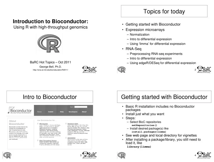2 http://iona.wi.mit.edu/bio/education/R2011/ Intro to Bioconductor Getting started with Bioconductor • Basic R installation includes no Bioconductor packages • Install just what you want • Steps: – Select BioC repositories setRepositories() – Install desired package(s) like install.packages(limma) • See web page and local directory for vignettes • See web page and local directory for vignettes • After installing a package/library, you still need to load it, like library(limma) 3 4

Expression microarrays Preprocessing Affymetrix arrays • One color or two color • Goals: • Probes can be short (25 mer) or long (60 mer) • Probes can be short (25-mer) or long (60-mer) – Normalize probes between arrays Normalize probes between arrays • A transcript may be represented by – Process mismatch probes (if present)? – One probe (Agilent) – Summarize probes into probeset values – Many probes (Affymetrix) grouped into a probeset • Common algorithms address these goals • Basic assumption: Intensity of color is correlated – MAS5 (original Affymetrix method) with gene-specific RNA abundance g p – RMA RMA • Today’s goals: – GCRMA – Measure relative RNA abundance • Choice of probeset definitions – Identify genes that differ between samples 5 6 Starting with Affy arrays in Bioc Absent/present calls • Install ‘affy’ and CDF (chip definition file) package • For Affymetrix arrays with mismatch probes too, for your array design o you a ay des g they can be compared to perfect match probes they can be compared to perfect match probes – Example for U133 Plus 2.0 array: – If the values are similar across the set, the probeset is install.packages(“affy”) called “absent” install.packages(“hg133plus2cdf”) • After reading a directory of CEL files as Data , • Go to directory with CEL files (containing probe-level data) and read them mas5calls = mas5calls(Data) # Do calls library(affy) # Get actual A/P matrix Data = ReadAffy() mas5calls.calls = exprs(mas5calls) • Preprocess into an expression set like write.table(mas5calls.calls, file=“APs.txt”, eset.mas5 = mas5(Data) quote=F, sep="\t") eset.rma = rma(Data) • You can choose if / how to use the calls. 7 8

Normalizing Agilent arrays 2-color Agilent arrays in Bioc • Goal is do maximize biological signal and minimize • Read arrays technical “noise” maData maData = read.maimages(dir(pattern = "txt"), read.maimages(dir(pattern txt ), • Major comparisons to optimize source="agilent“) – Within-array (red vs green channels) • Background correct (or not) – Between-arrays (all arrays to each other) maData.nobg.0 = backgroundCorrect(maData, • Other issues: method="none", offset=0) – If / how to use background levels • Normalize with loess – If / how to add an offset to all values MA.loess.0 = normalizeWithinArrays( • All methods rely on assumptions (expectations) All methods rely on assumptions (expectations) maData.nobg.0, method="loess") • Our favorite two-step method: • Normalize with Aquantile – Use loess for within-array normalization MA.loess.q.0 = normalizeBetweenArrays( – Use “Aquantile” normalization between arrays MA.loess.0, method="Aquantile") 9 10 Assaying differential expression Statistical testing with the t-test • Considers mean values and variability • Magnitude of fold change • Equation for the t-statistic in the Welch test: Equation for the t statistic in the Welch test: • Magnitude of variation between samples M it d f i ti b t l • Traditional statistical measures of confidence  mean mean … and then a p-value is calculated r g  – T-test t 2 r ; g = data sets to compare – Moderated t-test 2 s s g  s = standard deviation r – ANOVA n n n = no. of measurements – Paired t-test Paired t test r g g – Non-parametric test (Wilcoxon rank-sum test) • Disadvantages: • Other methods – Genes with small variances are more likely to make the cutoff – Works best with larger data sets than one usually has 11 12

Statistics with limma Limma: describing your experiment • Step 1: Fit a linear model for each gene FileName Target • Limma gets this GSM230387 OldSedentary – Starts with normalized expression matrix p information in two ways: information in two ways: GSM230397 GSM230397 OldTrained OldTrained – Estimates the variability of the data GSM230407 YoungSedentary Targets/design matrices: – Based on experimental design GSM230417 YoungTrained descriptions of RNA – Includes effect of each RNA source Old Old Young Young FileName sedentary trained sedentary trained – Command: lmFit() samples GSM230387 1 0 0 0 • Step 2: Perform moderated t-test for each gene GSM230397 0 1 0 0 Contrast matrix: list of GSM230407 0 0 1 0 – Based on desired comparisons desired comparisons GSM230417 0 0 0 1 – Calculates A (mean level across all arrays) and M (log2 – Calculates A (mean level across all arrays) and M (log2 fold change) OldTrained – YoungTrained - TrainedVsSedentary – T-test is moderated because variation is shared across OldSedentary YoungSedentary genes OldSedentary -1 0 -0.5 – Command: eBayes() OldTrained 1 0 0.5 YoungSedentary 0 -1 -0.5 13 YoungTrained 0 1 14 0.5 Multiple hypothesis testing RNA-Seq analysis basic steps • When performing one moderated t-test per • Preprocessing: probe, we have to be careful of false positives probe we have to be careful of false positives – Split by bar codes Split by bar codes – Quality control (and removal of poor-quality reads) • Solution: Adjust/correct (increase) p-values to – Remove adapters and linkers account for the high-throughput • Map to genome (maybe including gene models) • Most common method is False Discovery Rate • Count genes (or transcripts) • Definition/example of FDR: • Remove absent genes – If you select a FDR-adjust p-value threshold of 0.05, y j p , • Add offset (such as 1) Add ff t ( h 1) then you can expect 5% of your list of differentially – Prevent dividing by 0 expressed genes to be false positives – Moderate fold change of low-count genes • Do only as many statistical tests as necessary • Identify differentially expressed genes 15 16

Counts-based statistics Counts-based statistics Assaying differential expression • RNA-seq data representation is • Robust and confident analysis requires replication! replication! – Based on counts (integers), not continuous values – Based on counts (integers) not continuous values – Different from expression array data • Different R packages are available for experiments • Statistical test must be based on a corresponding distribution, such as the – without replication (but don’t believe the statistics) – Negative binomial – with replication – Poisson • With replication, BaRC has had success with • Expression data has the additional property of – edgeR having more variability than expected for these – DESeq distributions so is described as overdispersed – baySeq 17 18 Getting started in Bioc Intro to DESeq • Input data: matrix of counts • Requires raw counts, not RPKM values • Takes sample depth into consideration using T k l d th i t id ti i brain_1 brain_2 UHR_1 UHR_2 – Total read counts A1BG 46 65 96 107 A1CF 1 1 59 59 – Another more complex method • Install package(s) [just the first time] • Based on the negative binomial distribution • Call package • Extends (and may slightly outperform) edgeR Ex: library(DESeq) Ex: library(DESeq) • Calculates fold change and p-values • Read input matrix counts = read.delim(counts.txt, row.names=1) 19 20