
SLIDE 1
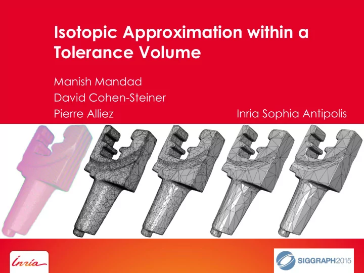
Isotopic Approximation within a Tolerance Volume
Manish Mandad David Cohen-Steiner Pierre Alliez
- 1
Tolerance Volume Manish Mandad David Cohen-Steiner Pierre Alliez - - PowerPoint PPT Presentation
Isotopic Approximation within a Tolerance Volume Manish Mandad David Cohen-Steiner Pierre Alliez Inria Sophia Antipolis - 1 Goals and Motivation - 2 Goals and Motivation Input: Tolerance volume of a surface geometry - 3 Goals and
+1 +1 +1 +1
+1 +1 +1 +1
+1 +1 +1 +1
Input Simplification Envelopes H = 60% Our Algorithm H = 10%
rδ ≥2δ During Simplification : Hausdorff distance between Z and boundary is enforced to be δ.