Today The multiplicative weights framework. Experts framework. n - PowerPoint PPT Presentation

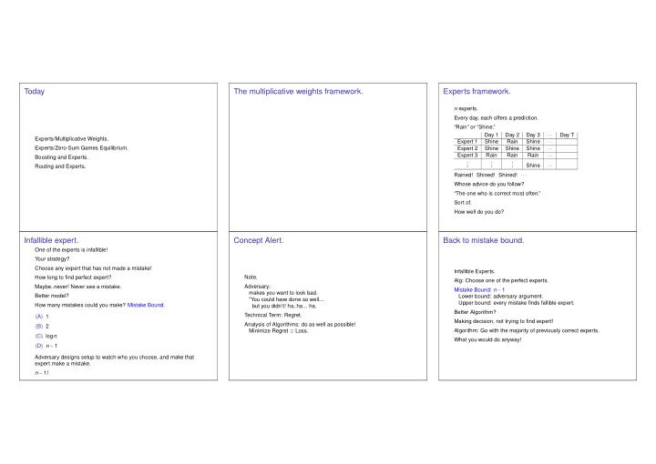
Today The multiplicative weights framework. Experts framework. n experts. Every day, each offers a prediction. “Rain” or “Shine.” Day 1 Day 2 Day 3 ··· Day T Experts/Multiplicative Weights. Expert 1 Shine Rain Shine ··· Experts/Zero-Sum Games Equilibrium. Expert 2 Shine Shine Shine ··· Expert 3 Rain Rain Rain ··· Boosting and Experts. . . . . . . . . . Shine ··· Routing and Experts. Rained! Shined! Shined! ··· Whose advice do you follow? “The one who is correct most often.” Sort of. How well do you do? Infallible expert. Concept Alert. Back to mistake bound. One of the experts is infallible! Your strategy? Choose any expert that has not made a mistake! Infallible Experts. How long to find perfect expert? Note. Alg: Choose one of the perfect experts. Maybe..never! Never see a mistake. Adversary: Mistake Bound: n − 1 makes you want to look bad. Better model? Lower bound: adversary argument. ”You could have done so well... Upper bound: every mistake finds fallible expert. How many mistakes could you make? Mistake Bound. but you didn’t! ha..ha... ha. Better Algorithm? Technical Term: Regret. (A) 1 Making decision, not trying to find expert! Analysis of Algorithms: do as well as possible! (B) 2 Algorithm: Go with the majority of previously correct experts. Minimize Regret ≡ Loss. (C) log n What you would do anyway! (D) n − 1 Adversary designs setup to watch who you choose, and make that expert make a mistake. n − 1!

Alg 2: find majority of the perfect Imperfect Experts Analysis: weighted majority How many mistakes could you make? 1. Initially: w i = 1. Goal: Best expert makes m mistakes. (A) 1 Goal? 2. Predict with Potential function: ∑ i w i . Initially n . (B) 2 Do as well as the best expert! weighted 1 For best expert, b , w b ≥ 2 m . majority of (C) log n Algorithm. Suggestions? Each mistake: experts. (D) n − 1 Go with majority? total weight of incorrect experts reduced by 3. w i → w i / 2 if factor of 1 − 1? − 2? 2 ? Penalize inaccurate experts? At most log n ! wrong. each incorrect expert weight multiplied by 1 2 ! Best expert is penalized the least. When alg makes a mistake, total weight decreases by | “perfect” experts | drops by a factor of two. factor of 1 2 ? factor of 3 4 ? 1. Initially: w i = 1. mistake → ≥ half weight with incorrect experts Initially n perfect experts ( ≥ 1 2 total. mistake → ≤ n / 2 perfect experts 2. Predict with weighted majority of experts. mistake → ≤ n / 4 perfect experts Mistake → potential function decreased by 3 4 . 3. w i → w i / 2 if wrong. . . . We have � 3 � M n . mistake → ≤ 1 perfect expert 1 2 m ≤ ∑ i w i ≤ 4 where M is number of algorithm mistakes. ≥ 1 perfect expert → at most log n mistakes! Analysis: continued. Best Analysis? Randomization!!!! � 3 � M n . 1 2 m ≤ ∑ i w i ≤ 4 Better approach? m - best expert mistakes M algorithm mistakes. Consider two experts: A,B Use? � 3 � M n . 1 2 m ≤ 4 Bad example? Randomization! Take log of both sides. Which is worse? That is, choose expert i with prob ∝ w i − m ≤ − M log ( 4 / 3 )+ log n . (A) A correct even days, B correct odd days Bad example: A,B,A,B,A... Solve for M . M ≤ ( m + log n ) / log ( 4 / 3 ) ≤ 2 . 4 ( m + log n ) (B) A correct first half of days, B correct second After a bit, A and B make nearly the same number of mistakes. Multiply by 1 − ε for incorrect experts... Choose each with approximately the same probabilty. Best expert peformance: T / 2 mistakes. � M n . ( 1 − ε ) m ≤ � 1 − ε Make a mistake around 1 / 2 of the time. Pattern (A): T − 1 mistakes. 2 Massage... Best expert makes T / 2 mistakes. Factor of (almost) two worse! M ≤ 2 ( 1 + ε ) m + 2ln n Roughly optimal! ε Approaches a factor of two of best expert performance!

Randomized analysis. Randomized algorithm Analysis Expert i loses ℓ t i ∈ [ 0 , 1 ] in round t. 1. Initially w i = 1 for expert i . ( 1 − ε ) L ∗ ≤ W ( T ) ≤ n ∏ t ( 1 − ε L t ) 2. Choose expert i with prob w i W , W = ∑ i w i . Some formulas: Take logs 3. w i ← w i ( 1 − ε ) ℓ t i ( L ∗ ) ln ( 1 − ε ) ≤ ln n + ∑ ln ( 1 − ε L t ) For ε ≤ 1 , x ∈ [ 0 , 1 ] , ( 1 + ε ) x ≤ ( 1 + ε x ) W ( t ) sum of w i at time t . W ( 0 ) = n Use − ε − ε 2 ≤ ln ( 1 − ε ) ≤ − ε ( 1 − ε ) x ≤ ( 1 − ε x ) Best expert, b , loses L ∗ total. → W ( T ) ≥ w b ≥ ( 1 − ε ) L ∗ . − ( L ∗ )( ε + ε 2 ) ≤ ln n − ε ∑ L t For ε ∈ [ 0 , 1 2 ] , w i ℓ t i And L t = ∑ i W expected loss of alg. in time t . − ε − ε 2 ≤ ln ( 1 − ε ) ≤ − ε ∑ t L t ≤ ( 1 + ε ) L ∗ + ln n Claim: W ( t + 1 ) ≤ W ( t )( 1 − ε L t ) Loss → weight loss. ε . ε − ε 2 ≤ ln ( 1 + ε ) ≤ ε Proof: ∑ t L t is total expected loss of algorithm. Proof Idea: ln ( 1 + x ) = x − x 2 2 + x 3 W ( t + 1 ) = ∑ ( 1 − ε ) ℓ t i w i ≤ ∑ = ∑ ( 1 − ε ℓ t w i ℓ t 3 −··· i ) w i w i − ε ∑ i Within ( 1 + ε ) ish of the best expert! i i i i No factor of 2 loss! � 1 − ε ∑ i w i ℓ t � = ∑ i w i ∑ i w i i = W ( t )( 1 − ε L t ) Gains. Summary: multiplicative weights. Two person zero sum games. m × n payoff matrix A . Row mixed strategy: x = ( x 1 ,..., x m ) . Why so negative? Framework: n experts, each loses different amount every day. Column mixed strategy: y = ( y 1 ,..., y n ) . Each day, each expert gives gain in [ 0 , 1 ] . Perfect Expert: log n mistakes. Payoff for strategy pair ( x , y ) : Multiplicative weights with ( 1 + ε ) g t i . Imperfect Expert: best makes m mistakes. p ( x , y ) = x t Ay Deterministic Strategy: 2 ( 1 + ε ) m + log n G ≥ ( 1 − ε ) G ∗ − log n ε That is, Real numbered losses: Best loses L ∗ total. ε where G ∗ is payoff of best expert. Randomized Strategy: ( 1 + ε ) L ∗ + log n � � � � = ∑ ε ∑ ∑ ∑ x i a i , j y j x i a i , j y j . Scaling: Strategy: i j j i Choose proportional to weights Not [ 0 , 1 ] , say [ 0 , ρ ] . Recall row minimizes, column maximizes. multiply weight by ( 1 − ε ) loss. Equilibrium pair: ( x ∗ , y ∗ ) ? L ≤ ( 1 + ε ) L ∗ + ρ log n Multiplicative weights framework! ε Applications next! ( x ∗ ) t Ay ∗ = max y ( x ∗ ) t Ay = min x x t Ay ∗ . (No better column strategy, no better row strategy.)

Equilibrium. Best Response Duality. x ( x t Ay ) . R = max min Column goes first: y y ( x t Ay ) . C = min x max Find y , where best row is not too low.. Equilibrium pair: ( x ∗ , y ∗ ) ? Weak Duality: R ≤ C . x ( x t Ay ) . R = max min p ( x , y ) = ( x ∗ ) t Ay ∗ = max Proof: Better to go second. y ( x ∗ ) t Ay = min x x t Ay ∗ . y At Equilibrium ( x ∗ , y ∗ ) , payoff v : Note: x can be ( 0 , 0 ,..., 1 ,... 0 ) . (No better column strategy, no better row strategy.) row payoffs ( Ay ∗ ) all ≥ v = ⇒ R ≥ v . Example: Roshambo. Value of R ? column payoffs ( ( x ∗ ) t A ) all ≤ v = ⇒ v ≥ C . No row is better: Row goes first: min i A ( i ) · y = ( x ∗ ) t Ay ∗ . 1 = ⇒ R ≥ C Find x , where best column is not high. Equilibrium = ⇒ R = C ! No column is better: max j ( A t ) ( j ) · x = ( x ∗ ) t Ay ∗ . y ( x t Ay ) . C = min x max Strong Duality: There is an equilibrium point! and R = C ! Doesn’t matter who plays first! Agin: y of form ( 0 , 0 ,..., 1 ,... 0 ) . Example: Roshambo. Value of C ? 1 A ( i ) is i th row. Proof of Equilibrium. Proof of approximate equilibrium. Games and experts Later. Well in just a minute..... Aproximate equilibrium ... Again: find ( x ∗ , y ∗ ) , such that How? C ( x ) = max y x t Ay ( max y x ∗ Ay ) − ( min x x ∗ Ay ∗ ) ≤ ε R ( y ) = min x x t Ay (A) Using geometry. C ( x ∗ ) R ( y ∗ ) ≤ ε − (B) Using a fixed point theorem. Always: R ( y ) ≤ C ( x ) ——————————————————————– Strategy pair: ( x , y ) (C) Using multiplicative weights. Experts Framework: n Experts, T days, L ∗ -total loss of best expert. Equilibrium: ( x , y ) (D) By the skin of my teeth. R ( y ) = C ( x ) → C ( x ) − R ( y ) = 0. Multiplicative Weights Method yields loss L where (C) ..and (D). Approximate Equilibrium: C ( x ) − R ( y ) ≤ ε . Not hard. Even easy. Still, head scratching happens. L ≤ ( 1 + ε ) L ∗ + log n ε With R ( y ) < C ( x ) → “Response y to x is within ε of best response” → “Response x to y is within ε of best response”