Timing attacks How typical software checks 16-byte authenticator: - - PowerPoint PPT Presentation

1

Timing attacks 1970s: TENEX operating system compares user-supplied string against secret password

• ne character at a time,

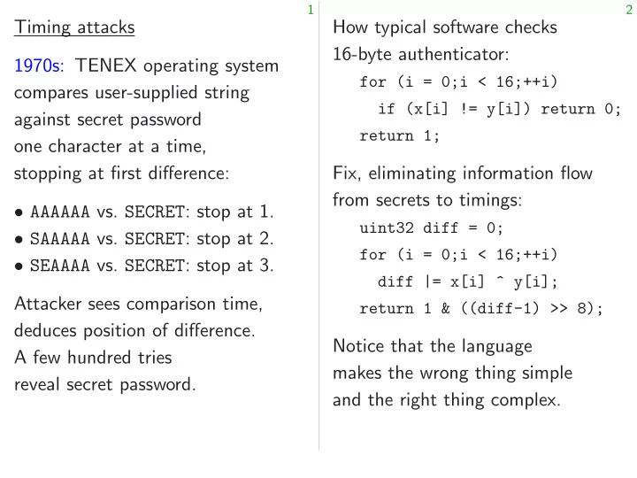
stopping at first difference:

• AAAAAA vs. SECRET: stop at 1.
• SAAAAA vs. SECRET: stop at 2.
• SEAAAA vs. SECRET: stop at 3.

Attacker sees comparison time, deduces position of difference. A few hundred tries reveal secret password.

2

How typical software checks 16-byte authenticator:

for (i = 0;i < 16;++i) if (x[i] != y[i]) return 0; return 1;

Fix, eliminating information flow from secrets to timings:

uint32 diff = 0; for (i = 0;i < 16;++i) diff |= x[i] ^ y[i]; return 1 & ((diff-1) >> 8);

Notice that the language makes the wrong thing simple and the right thing complex.

1

Timing attacks TENEX operating system res user-supplied string against secret password character at a time, stopping at first difference: AAAAAA vs. SECRET: stop at 1. SAAAAA vs. SECRET: stop at 2. SEAAAA vs. SECRET: stop at 3. er sees comparison time, deduces position of difference. hundred tries secret password.

2

How typical software checks 16-byte authenticator:

for (i = 0;i < 16;++i) if (x[i] != y[i]) return 0; return 1;

Fix, eliminating information flow from secrets to timings:

uint32 diff = 0; for (i = 0;i < 16;++i) diff |= x[i] ^ y[i]; return 1 & ((diff-1) >> 8);

Notice that the language makes the wrong thing simple and the right thing complex. Language “right” is So mistak

1

• perating system

user-supplied string password a time, difference: SECRET: stop at 1. SECRET: stop at 2. SECRET: stop at 3. comparison time,

• f difference.

tries password.

2

How typical software checks 16-byte authenticator:

for (i = 0;i < 16;++i) if (x[i] != y[i]) return 0; return 1;

Fix, eliminating information flow from secrets to timings:

uint32 diff = 0; for (i = 0;i < 16;++i) diff |= x[i] ^ y[i]; return 1 & ((diff-1) >> 8);

Notice that the language makes the wrong thing simple and the right thing complex. Language designer’s “right” is too weak So mistakes continue

1

system string difference: stop at 1. stop at 2. stop at 3. time, difference.

2

How typical software checks 16-byte authenticator:

for (i = 0;i < 16;++i) if (x[i] != y[i]) return 0; return 1;

Fix, eliminating information flow from secrets to timings:

uint32 diff = 0; for (i = 0;i < 16;++i) diff |= x[i] ^ y[i]; return 1 & ((diff-1) >> 8);

Notice that the language makes the wrong thing simple and the right thing complex. Language designer’s notion of “right” is too weak for securit So mistakes continue to happ

2

How typical software checks 16-byte authenticator:

for (i = 0;i < 16;++i) if (x[i] != y[i]) return 0; return 1;

Fix, eliminating information flow from secrets to timings:

uint32 diff = 0; for (i = 0;i < 16;++i) diff |= x[i] ^ y[i]; return 1 & ((diff-1) >> 8);

Notice that the language makes the wrong thing simple and the right thing complex.

3

Language designer’s notion of “right” is too weak for security. So mistakes continue to happen.

2

How typical software checks 16-byte authenticator:

for (i = 0;i < 16;++i) if (x[i] != y[i]) return 0; return 1;

Fix, eliminating information flow from secrets to timings:

uint32 diff = 0; for (i = 0;i < 16;++i) diff |= x[i] ^ y[i]; return 1 & ((diff-1) >> 8);

Notice that the language makes the wrong thing simple and the right thing complex.

3

Language designer’s notion of “right” is too weak for security. So mistakes continue to happen. One of many current examples, part of the reference software for CAESAR candidate CLOC:

/* compare the tag */ int i; for(i = 0;i < CRYPTO_ABYTES;i++) if(tag[i] != c[(*mlen) + i]){ return RETURN_TAG_NO_MATCH; } return RETURN_SUCCESS;

2

ypical software checks yte authenticator:

(i = 0;i < 16;++i) (x[i] != y[i]) return 0; return 1;

eliminating information flow secrets to timings:

uint32 diff = 0; (i = 0;i < 16;++i) diff |= x[i] ^ y[i]; return 1 & ((diff-1) >> 8);

that the language the wrong thing simple the right thing complex.

3

Language designer’s notion of “right” is too weak for security. So mistakes continue to happen. One of many current examples, part of the reference software for CAESAR candidate CLOC:

/* compare the tag */ int i; for(i = 0;i < CRYPTO_ABYTES;i++) if(tag[i] != c[(*mlen) + i]){ return RETURN_TAG_NO_MATCH; } return RETURN_SUCCESS;

Do timing Objection:

2

ware checks authenticator:

< 16;++i) y[i]) return 0;

information flow timings:

0; < 16;++i) x[i] ^ y[i]; ((diff-1) >> 8);

language wrong thing simple thing complex.

3

Language designer’s notion of “right” is too weak for security. So mistakes continue to happen. One of many current examples, part of the reference software for CAESAR candidate CLOC:

/* compare the tag */ int i; for(i = 0;i < CRYPTO_ABYTES;i++) if(tag[i] != c[(*mlen) + i]){ return RETURN_TAG_NO_MATCH; } return RETURN_SUCCESS;

Do timing attacks Objection: “Timings

2

checks

16;++i) return 0;

rmation flow

16;++i) y[i]; >> 8);

imple complex.

3

Language designer’s notion of “right” is too weak for security. So mistakes continue to happen. One of many current examples, part of the reference software for CAESAR candidate CLOC:

/* compare the tag */ int i; for(i = 0;i < CRYPTO_ABYTES;i++) if(tag[i] != c[(*mlen) + i]){ return RETURN_TAG_NO_MATCH; } return RETURN_SUCCESS;

Do timing attacks really work? Objection: “Timings are noisy!

3

Language designer’s notion of “right” is too weak for security. So mistakes continue to happen. One of many current examples, part of the reference software for CAESAR candidate CLOC:

/* compare the tag */ int i; for(i = 0;i < CRYPTO_ABYTES;i++) if(tag[i] != c[(*mlen) + i]){ return RETURN_TAG_NO_MATCH; } return RETURN_SUCCESS;

4

Do timing attacks really work? Objection: “Timings are noisy!”

3

Language designer’s notion of “right” is too weak for security. So mistakes continue to happen. One of many current examples, part of the reference software for CAESAR candidate CLOC:

/* compare the tag */ int i; for(i = 0;i < CRYPTO_ABYTES;i++) if(tag[i] != c[(*mlen) + i]){ return RETURN_TAG_NO_MATCH; } return RETURN_SUCCESS;

4

Do timing attacks really work? Objection: “Timings are noisy!” Answer #1: Does noise stop all attacks? To guarantee security, defender must block all information flow.

3

Language designer’s notion of “right” is too weak for security. So mistakes continue to happen. One of many current examples, part of the reference software for CAESAR candidate CLOC:

/* compare the tag */ int i; for(i = 0;i < CRYPTO_ABYTES;i++) if(tag[i] != c[(*mlen) + i]){ return RETURN_TAG_NO_MATCH; } return RETURN_SUCCESS;

4

Do timing attacks really work? Objection: “Timings are noisy!” Answer #1: Does noise stop all attacks? To guarantee security, defender must block all information flow. Answer #2: Attacker uses statistics to eliminate noise.

3

Language designer’s notion of “right” is too weak for security. So mistakes continue to happen. One of many current examples, part of the reference software for CAESAR candidate CLOC:

/* compare the tag */ int i; for(i = 0;i < CRYPTO_ABYTES;i++) if(tag[i] != c[(*mlen) + i]){ return RETURN_TAG_NO_MATCH; } return RETURN_SUCCESS;

4

Do timing attacks really work? Objection: “Timings are noisy!” Answer #1: Does noise stop all attacks? To guarantee security, defender must block all information flow. Answer #2: Attacker uses statistics to eliminate noise. Answer #3, what the 1970s attackers actually did: Cross page boundary, inducing page faults, to amplify timing signal.

3

Language designer’s notion of “right” is too weak for security. mistakes continue to happen.

• f many current examples,
• f the reference software for

CAESAR candidate CLOC:

compare the tag */ 0;i < CRYPTO_ABYTES;i++) if(tag[i] != c[(*mlen) + i]){ return RETURN_TAG_NO_MATCH; RETURN_SUCCESS;

4

Do timing attacks really work? Objection: “Timings are noisy!” Answer #1: Does noise stop all attacks? To guarantee security, defender must block all information flow. Answer #2: Attacker uses statistics to eliminate noise. Answer #3, what the 1970s attackers actually did: Cross page boundary, inducing page faults, to amplify timing signal. Examples 2005 Tromer–Osvik–Shamir: 65ms to used for 2013 AlF Thirteen: DTLS reco plaintext 2014 van steals Bitcoin

• f 25 Op

2016 Yarom–Genkin–Heninger “CacheBleed” key via timings

3

designer’s notion of eak for security. continue to happen. current examples, reference software for candidate CLOC:

tag */ CRYPTO_ABYTES;i++) c[(*mlen) + i]){ RETURN_TAG_NO_MATCH; RETURN_SUCCESS;

4

Do timing attacks really work? Objection: “Timings are noisy!” Answer #1: Does noise stop all attacks? To guarantee security, defender must block all information flow. Answer #2: Attacker uses statistics to eliminate noise. Answer #3, what the 1970s attackers actually did: Cross page boundary, inducing page faults, to amplify timing signal. Examples of successful 2005 Tromer–Osvik–Shamir: 65ms to steal Linux used for hard-disk 2013 AlFardan–Paterson Thirteen: breaking DTLS record proto plaintext using decryption 2014 van de Pol–Sma steals Bitcoin key from

• f 25 OpenSSL signatur

2016 Yarom–Genkin–Heninger “CacheBleed” steals key via timings of

3

notion of security. happen. examples, are for OC:

CRYPTO_ABYTES;i++) + i]){ RETURN_TAG_NO_MATCH;

4

Do timing attacks really work? Objection: “Timings are noisy!” Answer #1: Does noise stop all attacks? To guarantee security, defender must block all information flow. Answer #2: Attacker uses statistics to eliminate noise. Answer #3, what the 1970s attackers actually did: Cross page boundary, inducing page faults, to amplify timing signal. Examples of successful attacks: 2005 Tromer–Osvik–Shamir: 65ms to steal Linux AES key used for hard-disk encryption. 2013 AlFardan–Paterson “Lucky Thirteen: breaking the TLS DTLS record protocols” steals plaintext using decryption timings. 2014 van de Pol–Smart–Yarom steals Bitcoin key from timings

• f 25 OpenSSL signatures.

2016 Yarom–Genkin–Heninger “CacheBleed” steals RSA secret key via timings of OpenSSL.

4

Do timing attacks really work? Objection: “Timings are noisy!” Answer #1: Does noise stop all attacks? To guarantee security, defender must block all information flow. Answer #2: Attacker uses statistics to eliminate noise. Answer #3, what the 1970s attackers actually did: Cross page boundary, inducing page faults, to amplify timing signal.

5

Examples of successful attacks: 2005 Tromer–Osvik–Shamir: 65ms to steal Linux AES key used for hard-disk encryption. 2013 AlFardan–Paterson “Lucky Thirteen: breaking the TLS and DTLS record protocols” steals plaintext using decryption timings. 2014 van de Pol–Smart–Yarom steals Bitcoin key from timings

• f 25 OpenSSL signatures.

2016 Yarom–Genkin–Heninger “CacheBleed” steals RSA secret key via timings of OpenSSL.

4

timing attacks really work? Objection: “Timings are noisy!” er #1: noise stop all attacks? guarantee security, defender block all information flow. er #2: Attacker uses statistics to eliminate noise. er #3, what the attackers actually did: page boundary, inducing page faults, amplify timing signal.

5

Examples of successful attacks: 2005 Tromer–Osvik–Shamir: 65ms to steal Linux AES key used for hard-disk encryption. 2013 AlFardan–Paterson “Lucky Thirteen: breaking the TLS and DTLS record protocols” steals plaintext using decryption timings. 2014 van de Pol–Smart–Yarom steals Bitcoin key from timings

• f 25 OpenSSL signatures.

2016 Yarom–Genkin–Heninger “CacheBleed” steals RSA secret key via timings of OpenSSL. Constant-time ECDH com where a Key gene Signing: All of these Does timing Are there ECC ops? Do the underlying take variable

4

attacks really work? Timings are noisy!” all attacks? security, defender information flow. ttacker uses eliminate noise. what the actually did:

• undary,

aults, timing signal.

5

Examples of successful attacks: 2005 Tromer–Osvik–Shamir: 65ms to steal Linux AES key used for hard-disk encryption. 2013 AlFardan–Paterson “Lucky Thirteen: breaking the TLS and DTLS record protocols” steals plaintext using decryption timings. 2014 van de Pol–Smart–Yarom steals Bitcoin key from timings

• f 25 OpenSSL signatures.

2016 Yarom–Genkin–Heninger “CacheBleed” steals RSA secret key via timings of OpenSSL. Constant-time ECC ECDH computation: where a is your secret Key generation: a Signing: r → rB. All of these use secret Does timing leak this Are there any branches ECC ops? Point ops? Do the underlying take variable time?

4

• rk?

noisy!” attacks? defender flow. noise. did:

5

Examples of successful attacks: 2005 Tromer–Osvik–Shamir: 65ms to steal Linux AES key used for hard-disk encryption. 2013 AlFardan–Paterson “Lucky Thirteen: breaking the TLS and DTLS record protocols” steals plaintext using decryption timings. 2014 van de Pol–Smart–Yarom steals Bitcoin key from timings

• f 25 OpenSSL signatures.

2016 Yarom–Genkin–Heninger “CacheBleed” steals RSA secret key via timings of OpenSSL. Constant-time ECC ECDH computation: a; P → where a is your secret key. Key generation: a → aB. Signing: r → rB. All of these use secret data. Does timing leak this data? Are there any branches in ECC ops? Point ops? Field Do the underlying machine insns take variable time?

5

Examples of successful attacks: 2005 Tromer–Osvik–Shamir: 65ms to steal Linux AES key used for hard-disk encryption. 2013 AlFardan–Paterson “Lucky Thirteen: breaking the TLS and DTLS record protocols” steals plaintext using decryption timings. 2014 van de Pol–Smart–Yarom steals Bitcoin key from timings

• f 25 OpenSSL signatures.

2016 Yarom–Genkin–Heninger “CacheBleed” steals RSA secret key via timings of OpenSSL.

6

Constant-time ECC ECDH computation: a; P → aP where a is your secret key. Key generation: a → aB. Signing: r → rB. All of these use secret data. Does timing leak this data? Are there any branches in ECC ops? Point ops? Field ops? Do the underlying machine insns take variable time?

5

Examples of successful attacks: romer–Osvik–Shamir: to steal Linux AES key for hard-disk encryption. AlFardan–Paterson “Lucky Thirteen: breaking the TLS and record protocols” steals plaintext using decryption timings. van de Pol–Smart–Yarom Bitcoin key from timings OpenSSL signatures. arom–Genkin–Heninger “CacheBleed” steals RSA secret timings of OpenSSL.

6

Constant-time ECC ECDH computation: a; P → aP where a is your secret key. Key generation: a → aB. Signing: r → rB. All of these use secret data. Does timing leak this data? Are there any branches in ECC ops? Point ops? Field ops? Do the underlying machine insns take variable time? Recall left-to-right to compute using point

def scalarmult(n,P): if n == if n == R = scalarmult(n//2,P) R = R if n % return

Many branches NAF etc.

5

successful attacks: romer–Osvik–Shamir: Linux AES key rd-disk encryption. rdan–Paterson “Lucky reaking the TLS and rotocols” steals decryption timings.

• l–Smart–Yarom

ey from timings signatures. rom–Genkin–Heninger steals RSA secret

• f OpenSSL.

6

Constant-time ECC ECDH computation: a; P → aP where a is your secret key. Key generation: a → aB. Signing: r → rB. All of these use secret data. Does timing leak this data? Are there any branches in ECC ops? Point ops? Field ops? Do the underlying machine insns take variable time? Recall left-to-right to compute n; P → using point addition:

def scalarmult(n,P): if n == 0: return if n == 1: return R = scalarmult(n//2,P) R = R + R if n % 2: R = R return R

Many branches here. NAF etc. also use

5

attacks: romer–Osvik–Shamir: ey encryption. “Lucky TLS and steals timings. arom timings s. rom–Genkin–Heninger secret enSSL.

6

Constant-time ECC ECDH computation: a; P → aP where a is your secret key. Key generation: a → aB. Signing: r → rB. All of these use secret data. Does timing leak this data? Are there any branches in ECC ops? Point ops? Field ops? Do the underlying machine insns take variable time? Recall left-to-right binary metho to compute n; P → nP using point addition:

def scalarmult(n,P): if n == 0: return 0 if n == 1: return P R = scalarmult(n//2,P) R = R + R if n % 2: R = R + P return R

Many branches here. NAF etc. also use many branches.

6

Constant-time ECC ECDH computation: a; P → aP where a is your secret key. Key generation: a → aB. Signing: r → rB. All of these use secret data. Does timing leak this data? Are there any branches in ECC ops? Point ops? Field ops? Do the underlying machine insns take variable time?

7

Recall left-to-right binary method to compute n; P → nP using point addition:

def scalarmult(n,P): if n == 0: return 0 if n == 1: return P R = scalarmult(n//2,P) R = R + R if n % 2: R = R + P return R

Many branches here. NAF etc. also use many branches.

6

Constant-time ECC computation: a; P → aP a is your secret key. generation: a → aB. Signing: r → rB. these use secret data. timing leak this data? there any branches in

• ps? Point ops? Field ops?

the underlying machine insns variable time?

7

Recall left-to-right binary method to compute n; P → nP using point addition:

def scalarmult(n,P): if n == 0: return 0 if n == 1: return P R = scalarmult(n//2,P) R = R + R if n % 2: R = R + P return R

Many branches here. NAF etc. also use many branches. Even if each takes the (certainly total time If 2e−1 ≤ n has exactly number Particula usually indicates “Lattice compute positions

6

ECC utation: a; P → aP secret key. a → aB. . secret data. this data? ranches in

• ps? Field ops?

underlying machine insns time?

7

Recall left-to-right binary method to compute n; P → nP using point addition:

def scalarmult(n,P): if n == 0: return 0 if n == 1: return P R = scalarmult(n//2,P) R = R + R if n % 2: R = R + P return R

Many branches here. NAF etc. also use many branches. Even if each point takes the same amount (certainly not true total time depends If 2e−1 ≤ n < 2e and n has exactly w bits number of additions Particularly fast total usually indicates very “Lattice attacks” on compute the secret positions of very small

6

→ aP . data. data? Field ops? machine insns

7

Recall left-to-right binary method to compute n; P → nP using point addition:

def scalarmult(n,P): if n == 0: return 0 if n == 1: return P R = scalarmult(n//2,P) R = R + R if n % 2: R = R + P return R

Many branches here. NAF etc. also use many branches. Even if each point addition takes the same amount of time (certainly not true in Python), total time depends on n. If 2e−1 ≤ n < 2e and n has exactly w bits set: number of additions is e + w Particularly fast total time usually indicates very small n “Lattice attacks” on signatures compute the secret key given positions of very small nonces

7

Recall left-to-right binary method to compute n; P → nP using point addition:

def scalarmult(n,P): if n == 0: return 0 if n == 1: return P R = scalarmult(n//2,P) R = R + R if n % 2: R = R + P return R

Many branches here. NAF etc. also use many branches.

8

Even if each point addition takes the same amount of time (certainly not true in Python), total time depends on n. If 2e−1 ≤ n < 2e and n has exactly w bits set: number of additions is e + w − 2. Particularly fast total time usually indicates very small n. “Lattice attacks” on signatures compute the secret key given positions of very small nonces r.

7

left-to-right binary method compute n; P → nP point addition:

scalarmult(n,P): == 0: return 0 == 1: return P scalarmult(n//2,P) + R % 2: R = R + P return R

branches here.

• etc. also use many branches.

8

Even if each point addition takes the same amount of time (certainly not true in Python), total time depends on n. If 2e−1 ≤ n < 2e and n has exactly w bits set: number of additions is e + w − 2. Particularly fast total time usually indicates very small n. “Lattice attacks” on signatures compute the secret key given positions of very small nonces r. Even worse: CPUs do metadata Actual time affects, and detailed branch p Attacker

• ften sees

Exploited

7

left-to-right binary method → nP addition:

scalarmult(n,P): return 0 return P scalarmult(n//2,P) R + P

here. use many branches.

8

Even if each point addition takes the same amount of time (certainly not true in Python), total time depends on n. If 2e−1 ≤ n < 2e and n has exactly w bits set: number of additions is e + w − 2. Particularly fast total time usually indicates very small n. “Lattice attacks” on signatures compute the secret key given positions of very small nonces r. Even worse: CPUs do not try to metadata regarding Actual time for a b affects, and is affected detailed state of co branch predictor, etc. Attacker interacts

• ften sees pattern

Exploited in, e.g.,

7

method ranches.

8

Even if each point addition takes the same amount of time (certainly not true in Python), total time depends on n. If 2e−1 ≤ n < 2e and n has exactly w bits set: number of additions is e + w − 2. Particularly fast total time usually indicates very small n. “Lattice attacks” on signatures compute the secret key given positions of very small nonces r. Even worse: CPUs do not try to protect metadata regarding branches. Actual time for a branch affects, and is affected by, detailed state of code cache, branch predictor, etc. Attacker interacts with this state,

• ften sees pattern of branches.

Exploited in, e.g., Bitcoin attack.

8

Even if each point addition takes the same amount of time (certainly not true in Python), total time depends on n. If 2e−1 ≤ n < 2e and n has exactly w bits set: number of additions is e + w − 2. Particularly fast total time usually indicates very small n. “Lattice attacks” on signatures compute the secret key given positions of very small nonces r.

9

Even worse: CPUs do not try to protect metadata regarding branches. Actual time for a branch affects, and is affected by, detailed state of code cache, branch predictor, etc. Attacker interacts with this state,

• ften sees pattern of branches.

Exploited in, e.g., Bitcoin attack.

8

Even if each point addition takes the same amount of time (certainly not true in Python), total time depends on n. If 2e−1 ≤ n < 2e and n has exactly w bits set: number of additions is e + w − 2. Particularly fast total time usually indicates very small n. “Lattice attacks” on signatures compute the secret key given positions of very small nonces r.

9

Even worse: CPUs do not try to protect metadata regarding branches. Actual time for a branch affects, and is affected by, detailed state of code cache, branch predictor, etc. Attacker interacts with this state,

• ften sees pattern of branches.

Exploited in, e.g., Bitcoin attack. Confidence-inspiring solution: Avoid all data flow from secrets to branch conditions.

8

if each point addition the same amount of time (certainly not true in Python), time depends on n. ≤ n < 2e and exactly w bits set: er of additions is e + w − 2. rticularly fast total time indicates very small n. “Lattice attacks” on signatures compute the secret key given

• sitions of very small nonces r.

9

Even worse: CPUs do not try to protect metadata regarding branches. Actual time for a branch affects, and is affected by, detailed state of code cache, branch predictor, etc. Attacker interacts with this state,

• ften sees pattern of branches.

Exploited in, e.g., Bitcoin attack. Confidence-inspiring solution: Avoid all data flow from secrets to branch conditions. Double-and-add-alw Eliminate always computing

def scalarmult(n,b,P): if b == R = scalarmult(n//2,b-1,P) R2 = R S = [R2,R2 return

Works fo Always tak (including Use public

8

• int addition

amount of time true in Python), ds on n. and bits set: additions is e + w − 2. total time very small n. attacks” on signatures secret key given small nonces r.

9

Even worse: CPUs do not try to protect metadata regarding branches. Actual time for a branch affects, and is affected by, detailed state of code cache, branch predictor, etc. Attacker interacts with this state,

• ften sees pattern of branches.

Exploited in, e.g., Bitcoin attack. Confidence-inspiring solution: Avoid all data flow from secrets to branch conditions. Double-and-add-alw Eliminate branches always computing

def scalarmult(n,b,P): if b == 0: return R = scalarmult(n//2,b-1,P) R2 = R + R S = [R2,R2 + P] return S[n % 2]

Works for 0 ≤ n < Always takes 2b additions (including b doublings). Use public b: bits

8

addition time Python), w − 2. small n. signatures given nonces r.

9

Even worse: CPUs do not try to protect metadata regarding branches. Actual time for a branch affects, and is affected by, detailed state of code cache, branch predictor, etc. Attacker interacts with this state,

• ften sees pattern of branches.

Exploited in, e.g., Bitcoin attack. Confidence-inspiring solution: Avoid all data flow from secrets to branch conditions. Double-and-add-always Eliminate branches by always computing both results:

def scalarmult(n,b,P): if b == 0: return 0 R = scalarmult(n//2,b-1,P) R2 = R + R S = [R2,R2 + P] return S[n % 2]

Works for 0 ≤ n < 2b. Always takes 2b additions (including b doublings). Use public b: bits allowed in

9

Even worse: CPUs do not try to protect metadata regarding branches. Actual time for a branch affects, and is affected by, detailed state of code cache, branch predictor, etc. Attacker interacts with this state,

• ften sees pattern of branches.

Exploited in, e.g., Bitcoin attack. Confidence-inspiring solution: Avoid all data flow from secrets to branch conditions.

10

Double-and-add-always Eliminate branches by always computing both results:

def scalarmult(n,b,P): if b == 0: return 0 R = scalarmult(n//2,b-1,P) R2 = R + R S = [R2,R2 + P] return S[n % 2]

Works for 0 ≤ n < 2b. Always takes 2b additions (including b doublings). Use public b: bits allowed in n.

9

• rse:

do not try to protect metadata regarding branches. Actual time for a branch affects, and is affected by, detailed state of code cache, predictor, etc. er interacts with this state, sees pattern of branches. Exploited in, e.g., Bitcoin attack. Confidence-inspiring solution: all data flow from secrets to branch conditions.

10

Double-and-add-always Eliminate branches by always computing both results:

def scalarmult(n,b,P): if b == 0: return 0 R = scalarmult(n//2,b-1,P) R2 = R + R S = [R2,R2 + P] return S[n % 2]

Works for 0 ≤ n < 2b. Always takes 2b additions (including b doublings). Use public b: bits allowed in n. Another CPUs do metadata Actual time affects, and detailed store-to-load Exploited despite Intel claiming

9

to protect ding branches. a branch affected by, code cache, r, etc. interacts with this state, pattern of branches. e.g., Bitcoin attack. Confidence-inspiring solution: flow from ranch conditions.

10

Double-and-add-always Eliminate branches by always computing both results:

def scalarmult(n,b,P): if b == 0: return 0 R = scalarmult(n//2,b-1,P) R2 = R + R S = [R2,R2 + P] return S[n % 2]

Works for 0 ≤ n < 2b. Always takes 2b additions (including b doublings). Use public b: bits allowed in n. Another big problem: CPUs do not try to metadata regarding Actual time for x[i] affects, and is affected detailed state of data store-to-load forwa Exploited in, e.g., despite Intel and Op claiming their code

9

rotect ranches. cache, this state, ranches. attack. solution: conditions.

10

Double-and-add-always Eliminate branches by always computing both results:

def scalarmult(n,b,P): if b == 0: return 0 R = scalarmult(n//2,b-1,P) R2 = R + R S = [R2,R2 + P] return S[n % 2]

Works for 0 ≤ n < 2b. Always takes 2b additions (including b doublings). Use public b: bits allowed in n. Another big problem: CPUs do not try to protect metadata regarding array indices Actual time for x[i] affects, and is affected by, detailed state of data cache, store-to-load forwarder, etc. Exploited in, e.g., CacheBleed, despite Intel and OpenSSL claiming their code was safe.

10

Double-and-add-always Eliminate branches by always computing both results:

def scalarmult(n,b,P): if b == 0: return 0 R = scalarmult(n//2,b-1,P) R2 = R + R S = [R2,R2 + P] return S[n % 2]

Works for 0 ≤ n < 2b. Always takes 2b additions (including b doublings). Use public b: bits allowed in n.

11

Another big problem: CPUs do not try to protect metadata regarding array indices. Actual time for x[i] affects, and is affected by, detailed state of data cache, store-to-load forwarder, etc. Exploited in, e.g., CacheBleed, despite Intel and OpenSSL claiming their code was safe.

10

Double-and-add-always Eliminate branches by always computing both results:

def scalarmult(n,b,P): if b == 0: return 0 R = scalarmult(n//2,b-1,P) R2 = R + R S = [R2,R2 + P] return S[n % 2]

Works for 0 ≤ n < 2b. Always takes 2b additions (including b doublings). Use public b: bits allowed in n.

11

Another big problem: CPUs do not try to protect metadata regarding array indices. Actual time for x[i] affects, and is affected by, detailed state of data cache, store-to-load forwarder, etc. Exploited in, e.g., CacheBleed, despite Intel and OpenSSL claiming their code was safe. Confidence-inspiring solution: Avoid all data flow from secrets to memory addresses.

10

Double-and-add-always Eliminate branches by computing both results:

scalarmult(n,b,P): == 0: return 0 scalarmult(n//2,b-1,P) R + R [R2,R2 + P] return S[n % 2]

for 0 ≤ n < 2b. ys takes 2b additions (including b doublings). public b: bits allowed in n.

11

Another big problem: CPUs do not try to protect metadata regarding array indices. Actual time for x[i] affects, and is affected by, detailed state of data cache, store-to-load forwarder, etc. Exploited in, e.g., CacheBleed, despite Intel and OpenSSL claiming their code was safe. Confidence-inspiring solution: Avoid all data flow from secrets to memory addresses. Table lookups Always read Use bit op the desired

def scalarmult(n,b,P): if b == R = scalarmult(n//2,b-1,P) R2 = R S = [R2,R2 mask = return

10

Double-and-add-always nches by computing both results:

scalarmult(n,b,P): return 0 scalarmult(n//2,b-1,P) P] 2]

< 2b. additions doublings). bits allowed in n.

11

Another big problem: CPUs do not try to protect metadata regarding array indices. Actual time for x[i] affects, and is affected by, detailed state of data cache, store-to-load forwarder, etc. Exploited in, e.g., CacheBleed, despite Intel and OpenSSL claiming their code was safe. Confidence-inspiring solution: Avoid all data flow from secrets to memory addresses. Table lookups via a Always read all table Use bit operations the desired table entry:

def scalarmult(n,b,P): if b == 0: return R = scalarmult(n//2,b-1,P) R2 = R + R S = [R2,R2 + P] mask = -(n % 2) return S[0]^(mask&(S[1]^S[0]))

10

results:

scalarmult(n//2,b-1,P)

in n.

11

Another big problem: CPUs do not try to protect metadata regarding array indices. Actual time for x[i] affects, and is affected by, detailed state of data cache, store-to-load forwarder, etc. Exploited in, e.g., CacheBleed, despite Intel and OpenSSL claiming their code was safe. Confidence-inspiring solution: Avoid all data flow from secrets to memory addresses. Table lookups via arithmetic Always read all table entries. Use bit operations to select the desired table entry:

def scalarmult(n,b,P): if b == 0: return 0 R = scalarmult(n//2,b-1,P) R2 = R + R S = [R2,R2 + P] mask = -(n % 2) return S[0]^(mask&(S[1]^S[0]))

11

Another big problem: CPUs do not try to protect metadata regarding array indices. Actual time for x[i] affects, and is affected by, detailed state of data cache, store-to-load forwarder, etc. Exploited in, e.g., CacheBleed, despite Intel and OpenSSL claiming their code was safe. Confidence-inspiring solution: Avoid all data flow from secrets to memory addresses.

12

Table lookups via arithmetic Always read all table entries. Use bit operations to select the desired table entry:

def scalarmult(n,b,P): if b == 0: return 0 R = scalarmult(n//2,b-1,P) R2 = R + R S = [R2,R2 + P] mask = -(n % 2) return S[0]^(mask&(S[1]^S[0]))

11

Another big problem: do not try to protect metadata regarding array indices. Actual time for x[i] affects, and is affected by, detailed state of data cache, re-to-load forwarder, etc. Exploited in, e.g., CacheBleed, despite Intel and OpenSSL claiming their code was safe. Confidence-inspiring solution: all data flow from secrets to memory addresses.

12

Table lookups via arithmetic Always read all table entries. Use bit operations to select the desired table entry:

def scalarmult(n,b,P): if b == 0: return 0 R = scalarmult(n//2,b-1,P) R2 = R + R S = [R2,R2 + P] mask = -(n % 2) return S[0]^(mask&(S[1]^S[0]))

Width-2

def fixwin2(n,b,table): if b <= T = table[0] mask = T ^= ~mask mask = T ^= ~mask mask = T ^= ~mask R = fixwin2(n//4,b-2,table) R = R R = R return

11

roblem: to protect ding array indices. x[i] affected by, data cache, rwarder, etc. e.g., CacheBleed, OpenSSL de was safe. Confidence-inspiring solution: flow from memory addresses.

12

Table lookups via arithmetic Always read all table entries. Use bit operations to select the desired table entry:

def scalarmult(n,b,P): if b == 0: return 0 R = scalarmult(n//2,b-1,P) R2 = R + R S = [R2,R2 + P] mask = -(n % 2) return S[0]^(mask&(S[1]^S[0]))

Width-2 unsigned

def fixwin2(n,b,table): if b <= 0: return T = table[0] mask = (-(1 ^ (n T ^= ~mask & (T^table[1]) mask = (-(2 ^ (n T ^= ~mask & (T^table[2]) mask = (-(3 ^ (n T ^= ~mask & (T^table[3]) R = fixwin2(n//4,b-2,table) R = R + R R = R + R return R + T

11

rotect indices. cache, tc. CacheBleed, safe. solution: addresses.

12

Table lookups via arithmetic Always read all table entries. Use bit operations to select the desired table entry:

def scalarmult(n,b,P): if b == 0: return 0 R = scalarmult(n//2,b-1,P) R2 = R + R S = [R2,R2 + P] mask = -(n % 2) return S[0]^(mask&(S[1]^S[0]))

Width-2 unsigned fixed windo

def fixwin2(n,b,table): if b <= 0: return 0 T = table[0] mask = (-(1 ^ (n % 4))) T ^= ~mask & (T^table[1]) mask = (-(2 ^ (n % 4))) T ^= ~mask & (T^table[2]) mask = (-(3 ^ (n % 4))) T ^= ~mask & (T^table[3]) R = fixwin2(n//4,b-2,table) R = R + R R = R + R return R + T

12

Table lookups via arithmetic Always read all table entries. Use bit operations to select the desired table entry:

def scalarmult(n,b,P): if b == 0: return 0 R = scalarmult(n//2,b-1,P) R2 = R + R S = [R2,R2 + P] mask = -(n % 2) return S[0]^(mask&(S[1]^S[0]))

13

Width-2 unsigned fixed windows

def fixwin2(n,b,table): if b <= 0: return 0 T = table[0] mask = (-(1 ^ (n % 4))) >> 2 T ^= ~mask & (T^table[1]) mask = (-(2 ^ (n % 4))) >> 2 T ^= ~mask & (T^table[2]) mask = (-(3 ^ (n % 4))) >> 2 T ^= ~mask & (T^table[3]) R = fixwin2(n//4,b-2,table) R = R + R R = R + R return R + T

12

lookups via arithmetic ys read all table entries. bit operations to select desired table entry:

scalarmult(n,b,P): == 0: return 0 scalarmult(n//2,b-1,P) R + R [R2,R2 + P] = -(n % 2) return S[0]^(mask&(S[1]^S[0]))

13

Width-2 unsigned fixed windows

def fixwin2(n,b,table): if b <= 0: return 0 T = table[0] mask = (-(1 ^ (n % 4))) >> 2 T ^= ~mask & (T^table[1]) mask = (-(2 ^ (n % 4))) >> 2 T ^= ~mask & (T^table[2]) mask = (-(3 ^ (n % 4))) >> 2 T ^= ~mask & (T^table[3]) R = fixwin2(n//4,b-2,table) R = R + R R = R + R return R + T def scalarmult(n,b,P): P2 = P+P table return

Public branches, For b ∈ 2 Always b Always b Always 2 Can simila larger-width Unsigned Signed is

12

via arithmetic table entries. erations to select entry:

scalarmult(n,b,P): return 0 scalarmult(n//2,b-1,P) P] 2) S[0]^(mask&(S[1]^S[0]))

13

Width-2 unsigned fixed windows

def fixwin2(n,b,table): if b <= 0: return 0 T = table[0] mask = (-(1 ^ (n % 4))) >> 2 T ^= ~mask & (T^table[1]) mask = (-(2 ^ (n % 4))) >> 2 T ^= ~mask & (T^table[2]) mask = (-(3 ^ (n % 4))) >> 2 T ^= ~mask & (T^table[3]) R = fixwin2(n//4,b-2,table) R = R + R R = R + R return R + T def scalarmult(n,b,P): P2 = P+P table = [0,P,P2,P2+P] return fixwin2(n,b,table)

Public branches, public For b ∈ 2Z: Always b doublings. Always b=2 additions Always 2 additions Can similarly protect larger-width fixed windo Unsigned is slightly Signed is slightly faster.

12

rithmetic entries. select

scalarmult(n//2,b-1,P) S[0]^(mask&(S[1]^S[0]))

13

Width-2 unsigned fixed windows

def fixwin2(n,b,table): if b <= 0: return 0 T = table[0] mask = (-(1 ^ (n % 4))) >> 2 T ^= ~mask & (T^table[1]) mask = (-(2 ^ (n % 4))) >> 2 T ^= ~mask & (T^table[2]) mask = (-(3 ^ (n % 4))) >> 2 T ^= ~mask & (T^table[3]) R = fixwin2(n//4,b-2,table) R = R + R R = R + R return R + T def scalarmult(n,b,P): P2 = P+P table = [0,P,P2,P2+P] return fixwin2(n,b,table)

Public branches, public indices. For b ∈ 2Z: Always b doublings. Always b=2 additions of T. Always 2 additions for table. Can similarly protect larger-width fixed windows. Unsigned is slightly easier. Signed is slightly faster.

13

Width-2 unsigned fixed windows

def fixwin2(n,b,table): if b <= 0: return 0 T = table[0] mask = (-(1 ^ (n % 4))) >> 2 T ^= ~mask & (T^table[1]) mask = (-(2 ^ (n % 4))) >> 2 T ^= ~mask & (T^table[2]) mask = (-(3 ^ (n % 4))) >> 2 T ^= ~mask & (T^table[3]) R = fixwin2(n//4,b-2,table) R = R + R R = R + R return R + T

14

def scalarmult(n,b,P): P2 = P+P table = [0,P,P2,P2+P] return fixwin2(n,b,table)

Public branches, public indices. For b ∈ 2Z: Always b doublings. Always b=2 additions of T. Always 2 additions for table. Can similarly protect larger-width fixed windows. Unsigned is slightly easier. Signed is slightly faster.

13

Width-2 unsigned fixed windows

fixwin2(n,b,table): <= 0: return 0 table[0] = (-(1 ^ (n % 4))) >> 2 ~mask & (T^table[1]) = (-(2 ^ (n % 4))) >> 2 ~mask & (T^table[2]) = (-(3 ^ (n % 4))) >> 2 ~mask & (T^table[3]) fixwin2(n//4,b-2,table) + R + R return R + T

14

def scalarmult(n,b,P): P2 = P+P table = [0,P,P2,P2+P] return fixwin2(n,b,table)

Public branches, public indices. For b ∈ 2Z: Always b doublings. Always b=2 additions of T. Always 2 additions for table. Can similarly protect larger-width fixed windows. Unsigned is slightly easier. Signed is slightly faster. Fixed-base Obvious a → aB reuse n; P

13

unsigned fixed windows

fixwin2(n,b,table): return 0 (n % 4))) >> 2 (T^table[1]) (n % 4))) >> 2 (T^table[2]) (n % 4))) >> 2 (T^table[3]) fixwin2(n//4,b-2,table)

14

def scalarmult(n,b,P): P2 = P+P table = [0,P,P2,P2+P] return fixwin2(n,b,table)

Public branches, public indices. For b ∈ 2Z: Always b doublings. Always b=2 additions of T. Always 2 additions for table. Can similarly protect larger-width fixed windows. Unsigned is slightly easier. Signed is slightly faster. Fixed-base scalar multiplication Obvious way to handle a → aB and signing reuse n; P → nP from

13

windows

4))) >> 2 (T^table[1]) 4))) >> 2 (T^table[2]) 4))) >> 2 (T^table[3]) fixwin2(n//4,b-2,table)

14

def scalarmult(n,b,P): P2 = P+P table = [0,P,P2,P2+P] return fixwin2(n,b,table)

Public branches, public indices. For b ∈ 2Z: Always b doublings. Always b=2 additions of T. Always 2 additions for table. Can similarly protect larger-width fixed windows. Unsigned is slightly easier. Signed is slightly faster. Fixed-base scalar multiplication Obvious way to handle keygen a → aB and signing r → rB reuse n; P → nP from ECDH.

14

def scalarmult(n,b,P): P2 = P+P table = [0,P,P2,P2+P] return fixwin2(n,b,table)

Public branches, public indices. For b ∈ 2Z: Always b doublings. Always b=2 additions of T. Always 2 additions for table. Can similarly protect larger-width fixed windows. Unsigned is slightly easier. Signed is slightly faster.

15

Fixed-base scalar multiplication Obvious way to handle keygen a → aB and signing r → rB: reuse n; P → nP from ECDH.

14

def scalarmult(n,b,P): P2 = P+P table = [0,P,P2,P2+P] return fixwin2(n,b,table)

Public branches, public indices. For b ∈ 2Z: Always b doublings. Always b=2 additions of T. Always 2 additions for table. Can similarly protect larger-width fixed windows. Unsigned is slightly easier. Signed is slightly faster.

15

Fixed-base scalar multiplication Obvious way to handle keygen a → aB and signing r → rB: reuse n; P → nP from ECDH. Can do much better since B is a constant: standard base point. e.g. For b = 256: Compute (2128n1 + n0)B as n1B1 + n0B using double-scalar fixed windows, after precomputing B1 = 2128B. Fun exercise: For each k, try to minimize number of additions using k precomputed points.

14

scalarmult(n,b,P): P+P = [0,P,P2,P2+P] return fixwin2(n,b,table)

branches, public indices. ∈ 2Z: ys b doublings. ys b=2 additions of T. ys 2 additions for table. similarly protect rger-width fixed windows. Unsigned is slightly easier. is slightly faster.

15

Fixed-base scalar multiplication Obvious way to handle keygen a → aB and signing r → rB: reuse n; P → nP from ECDH. Can do much better since B is a constant: standard base point. e.g. For b = 256: Compute (2128n1 + n0)B as n1B1 + n0B using double-scalar fixed windows, after precomputing B1 = 2128B. Fun exercise: For each k, try to minimize number of additions using k precomputed points. Recall Chou 57164 cycles 63526 cycles 205741 cycles 159128 cycles ECDH is Verification somewhat (But batch Keygen is much faster Signing is depending

14

scalarmult(n,b,P): [0,P,P2,P2+P] fixwin2(n,b,table)

public indices. doublings. additions of T. additions for table. rotect fixed windows. slightly easier. faster.

15

Fixed-base scalar multiplication Obvious way to handle keygen a → aB and signing r → rB: reuse n; P → nP from ECDH. Can do much better since B is a constant: standard base point. e.g. For b = 256: Compute (2128n1 + n0)B as n1B1 + n0B using double-scalar fixed windows, after precomputing B1 = 2128B. Fun exercise: For each k, try to minimize number of additions using k precomputed points. Recall Chou timings: 57164 cycles for ke 63526 cycles for signature, 205741 cycles for verification, 159128 cycles for ECDH. ECDH is single-scala Verification is double-scala somewhat slower than (But batch verification Keygen is fixed-base much faster than ECDH. Signing is keygen plus depending on message

14

fixwin2(n,b,table)

indices. . table. ws.

15

Fixed-base scalar multiplication Obvious way to handle keygen a → aB and signing r → rB: reuse n; P → nP from ECDH. Can do much better since B is a constant: standard base point. e.g. For b = 256: Compute (2128n1 + n0)B as n1B1 + n0B using double-scalar fixed windows, after precomputing B1 = 2128B. Fun exercise: For each k, try to minimize number of additions using k precomputed points. Recall Chou timings: 57164 cycles for keygen, 63526 cycles for signature, 205741 cycles for verification, 159128 cycles for ECDH. ECDH is single-scalar mult. Verification is double-scalar mult, somewhat slower than ECDH. (But batch verification is faster.) Keygen is fixed-base scalar mult, much faster than ECDH. Signing is keygen plus overhead depending on message length.

15

Fixed-base scalar multiplication Obvious way to handle keygen a → aB and signing r → rB: reuse n; P → nP from ECDH. Can do much better since B is a constant: standard base point. e.g. For b = 256: Compute (2128n1 + n0)B as n1B1 + n0B using double-scalar fixed windows, after precomputing B1 = 2128B. Fun exercise: For each k, try to minimize number of additions using k precomputed points.

16

Recall Chou timings: 57164 cycles for keygen, 63526 cycles for signature, 205741 cycles for verification, 159128 cycles for ECDH. ECDH is single-scalar mult. Verification is double-scalar mult, somewhat slower than ECDH. (But batch verification is faster.) Keygen is fixed-base scalar mult, much faster than ECDH. Signing is keygen plus overhead depending on message length.

15

Fixed-base scalar multiplication Obvious way to handle keygen B and signing r → rB: n; P → nP from ECDH. do much better since B is constant: standard base point. r b = 256: Compute

1 + n0)B as n1B1 + n0B

double-scalar fixed windows, recomputing B1 = 2128B. exercise: For each k, try to minimize number of additions k precomputed points.

16

Recall Chou timings: 57164 cycles for keygen, 63526 cycles for signature, 205741 cycles for verification, 159128 cycles for ECDH. ECDH is single-scalar mult. Verification is double-scalar mult, somewhat slower than ECDH. (But batch verification is faster.) Keygen is fixed-base scalar mult, much faster than ECDH. Signing is keygen plus overhead depending on message length. Let’s move ECC verify S Point P; Q Field x1; x2 → Machine 32-bit multiplication Gates: AND,

15

r multiplication handle keygen signing r → rB: from ECDH. etter since B is standard base point. 256: Compute as n1B1 + n0B double-scalar fixed windows,

• mputing B1 = 2128B.

r each k, try to er of additions recomputed points.

16

Recall Chou timings: 57164 cycles for keygen, 63526 cycles for signature, 205741 cycles for verification, 159128 cycles for ECDH. ECDH is single-scalar mult. Verification is double-scalar mult, somewhat slower than ECDH. (But batch verification is faster.) Keygen is fixed-base scalar mult, much faster than ECDH. Signing is keygen plus overhead depending on message length. Let’s move down a ECC ops: e.g., verify SB = R + h windowing

• Point ops: e.g.,

P; Q → P + Q faster doubling

• Field ops: e.g.,

x1; x2 → x1x2 in F delayed

• Machine insns: e.g.,

32-bit multiplication pipelining

• Gates: e.g.,

AND, OR, XOR

15

multiplication eygen B: ECDH. B is point. Compute n0B windows, 2128B. try to additions

• ints.

16

Recall Chou timings: 57164 cycles for keygen, 63526 cycles for signature, 205741 cycles for verification, 159128 cycles for ECDH. ECDH is single-scalar mult. Verification is double-scalar mult, somewhat slower than ECDH. (But batch verification is faster.) Keygen is fixed-base scalar mult, much faster than ECDH. Signing is keygen plus overhead depending on message length. Let’s move down a level: ECC ops: e.g., verify SB = R + hA windowing etc.

• Point ops: e.g.,

P; Q → P + Q faster doubling etc

• Field ops: e.g.,

x1; x2 → x1x2 in Fp delayed carries etc.

• Machine insns: e.g.,

32-bit multiplication pipelining etc.

• Gates: e.g.,

AND, OR, XOR

16

Recall Chou timings: 57164 cycles for keygen, 63526 cycles for signature, 205741 cycles for verification, 159128 cycles for ECDH. ECDH is single-scalar mult. Verification is double-scalar mult, somewhat slower than ECDH. (But batch verification is faster.) Keygen is fixed-base scalar mult, much faster than ECDH. Signing is keygen plus overhead depending on message length.

17

Let’s move down a level: ECC ops: e.g., verify SB = R + hA windowing etc.

• Point ops: e.g.,

P; Q → P + Q faster doubling etc.

• Field ops: e.g.,

x1; x2 → x1x2 in Fp delayed carries etc.

• Machine insns: e.g.,

32-bit multiplication pipelining etc.

• Gates: e.g.,

AND, OR, XOR

16

Chou timings: cycles for keygen, cycles for signature, 205741 cycles for verification, 159128 cycles for ECDH. is single-scalar mult. erification is double-scalar mult, somewhat slower than ECDH. batch verification is faster.) Keygen is fixed-base scalar mult, faster than ECDH. Signing is keygen plus overhead ending on message length.

17

Let’s move down a level: ECC ops: e.g., verify SB = R + hA windowing etc.

• Point ops: e.g.,

P; Q → P + Q faster doubling etc.

• Field ops: e.g.,

x1; x2 → x1x2 in Fp delayed carries etc.

• Machine insns: e.g.,

32-bit multiplication pipelining etc.

• Gates: e.g.,

AND, OR, XOR Eliminating Have to

• f curve

How to efficiently additions Addition ((x1y2 + (y1y2 − uses exp

16

timings: keygen, signature, r verification, r ECDH. single-scalar mult. double-scalar mult, er than ECDH. verification is faster.) fixed-base scalar mult, than ECDH. eygen plus overhead message length.

17

Let’s move down a level: ECC ops: e.g., verify SB = R + hA windowing etc.

• Point ops: e.g.,

P; Q → P + Q faster doubling etc.

• Field ops: e.g.,

x1; x2 → x1x2 in Fp delayed carries etc.

• Machine insns: e.g.,

32-bit multiplication pipelining etc.

• Gates: e.g.,

AND, OR, XOR Eliminating divisions Have to do many additions

• f curve points: P;

How to efficiently additions into field Addition (x1; y1) + ((x1y2 + y1x2)=(1 (y1y2 − x1x2)=(1 uses expensive divisions.

16

signature, verification, mult. r mult, ECDH. faster.) r mult,

• verhead

length.

17

Let’s move down a level: ECC ops: e.g., verify SB = R + hA windowing etc.

• Point ops: e.g.,

P; Q → P + Q faster doubling etc.

• Field ops: e.g.,

x1; x2 → x1x2 in Fp delayed carries etc.

• Machine insns: e.g.,

32-bit multiplication pipelining etc.

• Gates: e.g.,

AND, OR, XOR Eliminating divisions Have to do many additions

• f curve points: P; Q → P +

How to efficiently decompose additions into field ops? Addition (x1; y1) + (x2; y2) = ((x1y2 + y1x2)=(1 + dx1x2y1 (y1y2 − x1x2)=(1 − dx1x2y1 uses expensive divisions.

17

Let’s move down a level: ECC ops: e.g., verify SB = R + hA windowing etc.

• Point ops: e.g.,

P; Q → P + Q faster doubling etc.

• Field ops: e.g.,

x1; x2 → x1x2 in Fp delayed carries etc.

• Machine insns: e.g.,

32-bit multiplication pipelining etc.

• Gates: e.g.,

AND, OR, XOR

18

Eliminating divisions Have to do many additions

• f curve points: P; Q → P + Q.

How to efficiently decompose additions into field ops? Addition (x1; y1) + (x2; y2) = ((x1y2 + y1x2)=(1 + dx1x2y1y2), (y1y2 − x1x2)=(1 − dx1x2y1y2)) uses expensive divisions.

17

Let’s move down a level: ECC ops: e.g., verify SB = R + hA windowing etc.

• Point ops: e.g.,

P; Q → P + Q faster doubling etc.

• Field ops: e.g.,

x1; x2 → x1x2 in Fp delayed carries etc.

• Machine insns: e.g.,

32-bit multiplication pipelining etc.

• Gates: e.g.,

AND, OR, XOR

18

Eliminating divisions Have to do many additions

• f curve points: P; Q → P + Q.

How to efficiently decompose additions into field ops? Addition (x1; y1) + (x2; y2) = ((x1y2 + y1x2)=(1 + dx1x2y1y2), (y1y2 − x1x2)=(1 − dx1x2y1y2)) uses expensive divisions. Better: postpone divisions and work with fractions. Represent (x; y) as (X : Y : Z) with x = X=Z, y = Y=Z, Z = 0.

17

move down a level: ECC ops: e.g., SB = R + hA windowing etc.

• int ops: e.g.,

Q → P + Q faster doubling etc.

• Field ops: e.g.,

→ x1x2 in Fp delayed carries etc.

• Machine insns: e.g.,

multiplication pipelining etc.

• Gates: e.g.,

AND, OR, XOR

18

Eliminating divisions Have to do many additions

• f curve points: P; Q → P + Q.

How to efficiently decompose additions into field ops? Addition (x1; y1) + (x2; y2) = ((x1y2 + y1x2)=(1 + dx1x2y1y2), (y1y2 − x1x2)=(1 − dx1x2y1y2)) uses expensive divisions. Better: postpone divisions and work with fractions. Represent (x; y) as (X : Y : Z) with x = X=Z, y = Y=Z, Z = 0. Addition handle fractions „X1 Z1 ; Y1 Z1

X1 Z1 Y2 Z2

1 + d X

Z Y1 Z1 Y2 Z2

1 − d X

Z

17

a level: e.g., hA windowing etc. e.g., Q faster doubling etc. e.g., in Fp ed carries etc. e.g., multiplication elining etc. e.g., OR

18

Eliminating divisions Have to do many additions

• f curve points: P; Q → P + Q.

How to efficiently decompose additions into field ops? Addition (x1; y1) + (x2; y2) = ((x1y2 + y1x2)=(1 + dx1x2y1y2), (y1y2 − x1x2)=(1 − dx1x2y1y2)) uses expensive divisions. Better: postpone divisions and work with fractions. Represent (x; y) as (X : Y : Z) with x = X=Z, y = Y=Z, Z = 0. Addition now has to handle fractions as „X1 Z1 ; Y1 Z1 « + „X2 Z2

X1 Z1 Y2 Z2 + Y1 Z1 X2 Z2

1 + d X1

Z1 X2 Z2 Y1 Z1 Y2 Z2 Y1 Z1 Y2 Z2 − X1 Z1 X2 Z2

1 − d X1

Z1 X2 Z2 Y1 Z1 Y2 Z2

17

tc. etc. etc.

18

Eliminating divisions Have to do many additions

• f curve points: P; Q → P + Q.

How to efficiently decompose additions into field ops? Addition (x1; y1) + (x2; y2) = ((x1y2 + y1x2)=(1 + dx1x2y1y2), (y1y2 − x1x2)=(1 − dx1x2y1y2)) uses expensive divisions. Better: postpone divisions and work with fractions. Represent (x; y) as (X : Y : Z) with x = X=Z, y = Y=Z, Z = 0. Addition now has to handle fractions as input: „X1 Z1 ; Y1 Z1 « + „X2 Z2 ; Y2 Z2 « =

X1 Z1 Y2 Z2 + Y1 Z1 X2 Z2

1 + d X1

Z1 X2 Z2 Y1 Z1 Y2 Z2

,

Y1 Z1 Y2 Z2 − X1 Z1 X2 Z2

1 − d X1

Z1 X2 Z2 Y1 Z1 Y2 Z2

! =

18

Eliminating divisions Have to do many additions

• f curve points: P; Q → P + Q.

How to efficiently decompose additions into field ops? Addition (x1; y1) + (x2; y2) = ((x1y2 + y1x2)=(1 + dx1x2y1y2), (y1y2 − x1x2)=(1 − dx1x2y1y2)) uses expensive divisions. Better: postpone divisions and work with fractions. Represent (x; y) as (X : Y : Z) with x = X=Z, y = Y=Z, Z = 0.

19

Addition now has to handle fractions as input: „X1 Z1 ; Y1 Z1 « + „X2 Z2 ; Y2 Z2 « =

X1 Z1 Y2 Z2 + Y1 Z1 X2 Z2

1 + d X1

Z1 X2 Z2 Y1 Z1 Y2 Z2

,

Y1 Z1 Y2 Z2 − X1 Z1 X2 Z2

1 − d X1

Z1 X2 Z2 Y1 Z1 Y2 Z2

! =

18

Eliminating divisions Have to do many additions

• f curve points: P; Q → P + Q.

How to efficiently decompose additions into field ops? Addition (x1; y1) + (x2; y2) = ((x1y2 + y1x2)=(1 + dx1x2y1y2), (y1y2 − x1x2)=(1 − dx1x2y1y2)) uses expensive divisions. Better: postpone divisions and work with fractions. Represent (x; y) as (X : Y : Z) with x = X=Z, y = Y=Z, Z = 0.

19

Addition now has to handle fractions as input: „X1 Z1 ; Y1 Z1 « + „X2 Z2 ; Y2 Z2 « =

X1 Z1 Y2 Z2 + Y1 Z1 X2 Z2

1 + d X1

Z1 X2 Z2 Y1 Z1 Y2 Z2

,

Y1 Z1 Y2 Z2 − X1 Z1 X2 Z2

1 − d X1

Z1 X2 Z2 Y1 Z1 Y2 Z2

! = Z1Z2(X1Y2 + Y1X2) Z2

1Z2 2 + dX1X2Y1Y2

, Z1Z2(Y1Y2 − X1X2) Z2

1Z2 2 − dX1X2Y1Y2

!

18

Eliminating divisions to do many additions curve points: P; Q → P + Q. to efficiently decompose additions into field ops? Addition (x1; y1) + (x2; y2) = + y1x2)=(1 + dx1x2y1y2), − x1x2)=(1 − dx1x2y1y2)) expensive divisions. Better: postpone divisions

• rk with fractions.

resent (x; y) as (X : Y : Z) = X=Z, y = Y=Z, Z = 0.

19

Addition now has to handle fractions as input: „X1 Z1 ; Y1 Z1 « + „X2 Z2 ; Y2 Z2 « =

X1 Z1 Y2 Z2 + Y1 Z1 X2 Z2

1 + d X1

Z1 X2 Z2 Y1 Z1 Y2 Z2

,

Y1 Z1 Y2 Z2 − X1 Z1 X2 Z2

1 − d X1

Z1 X2 Z2 Y1 Z1 Y2 Z2

! = Z1Z2(X1Y2 + Y1X2) Z2

1Z2 2 + dX1X2Y1Y2

, Z1Z2(Y1Y2 − X1X2) Z2

1Z2 2 − dX1X2Y1Y2

! i.e. „X1 Z1 = „X3 Z3 ; where F = Z2

1Z

G = Z2

1Z

X3 = Z1 Y3 = Z1Z Z3 = FG Input to X1; Y1; Z Output from X3; Y3; Z

18

divisions many additions P; Q → P + Q. efficiently decompose field ops? + (x2; y2) = (1 + dx1x2y1y2), (1 − dx1x2y1y2)) divisions.

• ne divisions

fractions. as (X : Y : Z) = Y=Z, Z = 0.

19

Addition now has to handle fractions as input: „X1 Z1 ; Y1 Z1 « + „X2 Z2 ; Y2 Z2 « =

X1 Z1 Y2 Z2 + Y1 Z1 X2 Z2

1 + d X1

Z1 X2 Z2 Y1 Z1 Y2 Z2

,

Y1 Z1 Y2 Z2 − X1 Z1 X2 Z2

1 − d X1

Z1 X2 Z2 Y1 Z1 Y2 Z2

! = Z1Z2(X1Y2 + Y1X2) Z2

1Z2 2 + dX1X2Y1Y2

, Z1Z2(Y1Y2 − X1X2) Z2

1Z2 2 − dX1X2Y1Y2

! i.e. „X1 Z1 ; Y1 Z1 « + „ = „X3 Z3 ; Y3 Z3 « where F = Z2

1Z2 2 − dX1X

G = Z2

1Z2 2 + dX1X

X3 = Z1Z2(X1Y2 + Y3 = Z1Z2(Y1Y2 − Z3 = FG. Input to addition algo X1; Y1; Z1; X2; Y2; Z Output from addition X3; Y3; Z3. No divisions

18

additions + Q.

• se

) = y1y2), y1y2)) : Z) Z = 0.

19

Addition now has to handle fractions as input: „X1 Z1 ; Y1 Z1 « + „X2 Z2 ; Y2 Z2 « =

X1 Z1 Y2 Z2 + Y1 Z1 X2 Z2

1 + d X1

Z1 X2 Z2 Y1 Z1 Y2 Z2

,

Y1 Z1 Y2 Z2 − X1 Z1 X2 Z2

1 − d X1

Z1 X2 Z2 Y1 Z1 Y2 Z2

! = Z1Z2(X1Y2 + Y1X2) Z2

1Z2 2 + dX1X2Y1Y2

, Z1Z2(Y1Y2 − X1X2) Z2

1Z2 2 − dX1X2Y1Y2

! i.e. „X1 Z1 ; Y1 Z1 « + „X2 Z2 ; Y2 Z2 « = „X3 Z3 ; Y3 Z3 « where F = Z2

1Z2 2 − dX1X2Y1Y2,

G = Z2

1Z2 2 + dX1X2Y1Y2,

X3 = Z1Z2(X1Y2 + Y1X2)F, Y3 = Z1Z2(Y1Y2 − X1X2)G, Z3 = FG. Input to addition algorithm: X1; Y1; Z1; X2; Y2; Z2. Output from addition algorithm: X3; Y3; Z3. No divisions needed!

19

Addition now has to handle fractions as input: „X1 Z1 ; Y1 Z1 « + „X2 Z2 ; Y2 Z2 « =

X1 Z1 Y2 Z2 + Y1 Z1 X2 Z2

1 + d X1

Z1 X2 Z2 Y1 Z1 Y2 Z2

,

Y1 Z1 Y2 Z2 − X1 Z1 X2 Z2

1 − d X1

Z1 X2 Z2 Y1 Z1 Y2 Z2

! = Z1Z2(X1Y2 + Y1X2) Z2

1Z2 2 + dX1X2Y1Y2

, Z1Z2(Y1Y2 − X1X2) Z2

1Z2 2 − dX1X2Y1Y2

!

20

i.e. „X1 Z1 ; Y1 Z1 « + „X2 Z2 ; Y2 Z2 « = „X3 Z3 ; Y3 Z3 « where F = Z2

1Z2 2 − dX1X2Y1Y2,

G = Z2

1Z2 2 + dX1X2Y1Y2,

X3 = Z1Z2(X1Y2 + Y1X2)F, Y3 = Z1Z2(Y1Y2 − X1X2)G, Z3 = FG. Input to addition algorithm: X1; Y1; Z1; X2; Y2; Z2. Output from addition algorithm: X3; Y3; Z3. No divisions needed!

19

Addition now has to fractions as input: Y1 Z1 « + „X2 Z2 ; Y2 Z2 « =

Y2 Z2 + Y1 Z1 X2 Z2

d X1

Z1 X2 Z2 Y1 Z1 Y2 Z2

,

Y2 Z2 − X1 Z1 X2 Z2

d X1

Z1 X2 Z2 Y1 Z1 Y2 Z2

! =

2(X1Y2 + Y1X2) 2 2 + dX1X2Y1Y2

,

2(Y1Y2 − X1X2) 2 2 − dX1X2Y1Y2

!

20

i.e. „X1 Z1 ; Y1 Z1 « + „X2 Z2 ; Y2 Z2 « = „X3 Z3 ; Y3 Z3 « where F = Z2

1Z2 2 − dX1X2Y1Y2,

G = Z2

1Z2 2 + dX1X2Y1Y2,

X3 = Z1Z2(X1Y2 + Y1X2)F, Y3 = Z1Z2(Y1Y2 − X1X2)G, Z3 = FG. Input to addition algorithm: X1; Y1; Z1; X2; Y2; Z2. Output from addition algorithm: X3; Y3; Z3. No divisions needed! Eliminate to save multiplications: A = Z1 · C = X1 · D = Y1 · E = d · C F = B − X3 = A · Y3 = A · Z3 = F · Cost: 11 M; S are Choose small

19

has to as input: X2 Z2 ; Y2 Z2 « =

2 2

Y2 Z2

,

2 2

Y2 Z2

! = Y1X2)

2Y1Y2

, X1X2)

2Y1Y2

!

20

i.e. „X1 Z1 ; Y1 Z1 « + „X2 Z2 ; Y2 Z2 « = „X3 Z3 ; Y3 Z3 « where F = Z2

1Z2 2 − dX1X2Y1Y2,

G = Z2

1Z2 2 + dX1X2Y1Y2,

X3 = Z1Z2(X1Y2 + Y1X2)F, Y3 = Z1Z2(Y1Y2 − X1X2)G, Z3 = FG. Input to addition algorithm: X1; Y1; Z1; X2; Y2; Z2. Output from addition algorithm: X3; Y3; Z3. No divisions needed! Eliminate common to save multiplications: A = Z1 · Z2; B = A C = X1 · X2; D = Y1 · Y2; E = d · C · D; F = B − E; G = B X3 = A · F · (X1 · Y Y3 = A · G · (D − C Z3 = F · G. Cost: 11M + 1S + M; S are costs of mult, Choose small d for

19

=

20

i.e. „X1 Z1 ; Y1 Z1 « + „X2 Z2 ; Y2 Z2 « = „X3 Z3 ; Y3 Z3 « where F = Z2

1Z2 2 − dX1X2Y1Y2,

G = Z2

1Z2 2 + dX1X2Y1Y2,

X3 = Z1Z2(X1Y2 + Y1X2)F, Y3 = Z1Z2(Y1Y2 − X1X2)G, Z3 = FG. Input to addition algorithm: X1; Y1; Z1; X2; Y2; Z2. Output from addition algorithm: X3; Y3; Z3. No divisions needed! Eliminate common subexpressions to save multiplications: A = Z1 · Z2; B = A2; C = X1 · X2; D = Y1 · Y2; E = d · C · D; F = B − E; G = B + E; X3 = A · F · (X1 · Y2 + Y1 · X Y3 = A · G · (D − C); Z3 = F · G. Cost: 11M + 1S + 1Md where M; S are costs of mult, squa Choose small d for cheap M

20

i.e. „X1 Z1 ; Y1 Z1 « + „X2 Z2 ; Y2 Z2 « = „X3 Z3 ; Y3 Z3 « where F = Z2

1Z2 2 − dX1X2Y1Y2,

G = Z2

1Z2 2 + dX1X2Y1Y2,

X3 = Z1Z2(X1Y2 + Y1X2)F, Y3 = Z1Z2(Y1Y2 − X1X2)G, Z3 = FG. Input to addition algorithm: X1; Y1; Z1; X2; Y2; Z2. Output from addition algorithm: X3; Y3; Z3. No divisions needed!

21

Eliminate common subexpressions to save multiplications: A = Z1 · Z2; B = A2; C = X1 · X2; D = Y1 · Y2; E = d · C · D; F = B − E; G = B + E; X3 = A · F · (X1 · Y2 + Y1 · X2); Y3 = A · G · (D − C); Z3 = F · G. Cost: 11M + 1S + 1Md where M; S are costs of mult, square. Choose small d for cheap Md.

20

1

Z1 ; Y1 Z1 « + „X2 Z2 ; Y2 Z2 «

3 ; Y3

Z3 «

2 1Z2 2 − dX1X2Y1Y2, 2 1Z2 2 + dX1X2Y1Y2,

Z1Z2(X1Y2 + Y1X2)F,

1Z2(Y1Y2 − X1X2)G,

G. to addition algorithm: ; Z1; X2; Y2; Z2. Output from addition algorithm: ; Z3. No divisions needed!

21

Eliminate common subexpressions to save multiplications: A = Z1 · Z2; B = A2; C = X1 · X2; D = Y1 · Y2; E = d · C · D; F = B − E; G = B + E; X3 = A · F · (X1 · Y2 + Y1 · X2); Y3 = A · G · (D − C); Z3 = F · G. Cost: 11M + 1S + 1Md where M; S are costs of mult, square. Choose small d for cheap Md. Can do b Obvious compute

• f polys

C = X1 · D = Y1 · M = X1

20

„X2 Z2 ; Y2 Z2 «

1X2Y1Y2, 1X2Y1Y2, 2 + Y1X2)F,

− X1X2)G, algorithm: ; Z2. dition algorithm: divisions needed!

21

Eliminate common subexpressions to save multiplications: A = Z1 · Z2; B = A2; C = X1 · X2; D = Y1 · Y2; E = d · C · D; F = B − E; G = B + E; X3 = A · F · (X1 · Y2 + Y1 · X2); Y3 = A · G · (D − C); Z3 = F · G. Cost: 11M + 1S + 1Md where M; S are costs of mult, square. Choose small d for cheap Md. Can do better: 10M Obvious 4M metho compute product C

• f polys X1 + Y1t,

C = X1 · X2; D = Y1 · Y2; M = X1 · Y2 + Y1 ·

20

« F, G, rithm: rithm: needed!

21

Eliminate common subexpressions to save multiplications: A = Z1 · Z2; B = A2; C = X1 · X2; D = Y1 · Y2; E = d · C · D; F = B − E; G = B + E; X3 = A · F · (X1 · Y2 + Y1 · X2); Y3 = A · G · (D − C); Z3 = F · G. Cost: 11M + 1S + 1Md where M; S are costs of mult, square. Choose small d for cheap Md. Can do better: 10M + 1S + Obvious 4M method to compute product C + Mt +

• f polys X1 + Y1t, X2 + Y2t:

C = X1 · X2; D = Y1 · Y2; M = X1 · Y2 + Y1 · X2.

21

Eliminate common subexpressions to save multiplications: A = Z1 · Z2; B = A2; C = X1 · X2; D = Y1 · Y2; E = d · C · D; F = B − E; G = B + E; X3 = A · F · (X1 · Y2 + Y1 · X2); Y3 = A · G · (D − C); Z3 = F · G. Cost: 11M + 1S + 1Md where M; S are costs of mult, square. Choose small d for cheap Md.

22

Can do better: 10M + 1S + 1Md. Obvious 4M method to compute product C + Mt + Dt2

• f polys X1 + Y1t, X2 + Y2t:

C = X1 · X2; D = Y1 · Y2; M = X1 · Y2 + Y1 · X2.

21

Eliminate common subexpressions to save multiplications: A = Z1 · Z2; B = A2; C = X1 · X2; D = Y1 · Y2; E = d · C · D; F = B − E; G = B + E; X3 = A · F · (X1 · Y2 + Y1 · X2); Y3 = A · G · (D − C); Z3 = F · G. Cost: 11M + 1S + 1Md where M; S are costs of mult, square. Choose small d for cheap Md.

22

Can do better: 10M + 1S + 1Md. Obvious 4M method to compute product C + Mt + Dt2

• f polys X1 + Y1t, X2 + Y2t:

C = X1 · X2; D = Y1 · Y2; M = X1 · Y2 + Y1 · X2. Karatsuba’s 3M method: C = X1 · X2; D = Y1 · Y2; M = (X1 +Y1)·(X2 +Y2)−C −D.

21

Eliminate common subexpressions save multiplications:

1 · Z2; B = A2; 1 · X2; 1 · Y2;

· C · D; − E; G = B + E; A · F · (X1 · Y2 + Y1 · X2); · G · (D − C); · G. 11M + 1S + 1Md where re costs of mult, square.

• se small d for cheap Md.

22

Can do better: 10M + 1S + 1Md. Obvious 4M method to compute product C + Mt + Dt2

• f polys X1 + Y1t, X2 + Y2t:

C = X1 · X2; D = Y1 · Y2; M = X1 · Y2 + Y1 · X2. Karatsuba’s 3M method: C = X1 · X2; D = Y1 · Y2; M = (X1 +Y1)·(X2 +Y2)−C −D. Faster doublin (x1; y1) + ((x1y1+y (y1y1−x ((2x1y1)= (y2

1 −x2 1

21

• n subexpressions

multiplications: = A2; B + E; · Y2 + Y1 · X2); − C); + 1Md where

• f mult, square.

for cheap Md.

22

Can do better: 10M + 1S + 1Md. Obvious 4M method to compute product C + Mt + Dt2

• f polys X1 + Y1t, X2 + Y2t:

C = X1 · X2; D = Y1 · Y2; M = X1 · Y2 + Y1 · X2. Karatsuba’s 3M method: C = X1 · X2; D = Y1 · Y2; M = (X1 +Y1)·(X2 +Y2)−C −D. Faster doubling (x1; y1) + (x1; y1) = ((x1y1+y1x1)=(1+ (y1y1−x1x1)=(1− ((2x1y1)=(1 + dx2

1

(y2

1 −x2 1)=(1 − dx

21

ressions · X2); where square. Md.

22

Can do better: 10M + 1S + 1Md. Obvious 4M method to compute product C + Mt + Dt2

• f polys X1 + Y1t, X2 + Y2t:

C = X1 · X2; D = Y1 · Y2; M = X1 · Y2 + Y1 · X2. Karatsuba’s 3M method: C = X1 · X2; D = Y1 · Y2; M = (X1 +Y1)·(X2 +Y2)−C −D. Faster doubling (x1; y1) + (x1; y1) = ((x1y1+y1x1)=(1+dx1x1y1y1 (y1y1−x1x1)=(1−dx1x1y1y1 ((2x1y1)=(1 + dx2

1y2 1 ),

(y2

1 −x2 1)=(1 − dx2 1y2 1 )).

22

Can do better: 10M + 1S + 1Md. Obvious 4M method to compute product C + Mt + Dt2

• f polys X1 + Y1t, X2 + Y2t:

C = X1 · X2; D = Y1 · Y2; M = X1 · Y2 + Y1 · X2. Karatsuba’s 3M method: C = X1 · X2; D = Y1 · Y2; M = (X1 +Y1)·(X2 +Y2)−C −D.

23

Faster doubling (x1; y1) + (x1; y1) = ((x1y1+y1x1)=(1+dx1x1y1y1), (y1y1−x1x1)=(1−dx1x1y1y1)) = ((2x1y1)=(1 + dx2

1y2 1 ),

(y2

1 −x2 1)=(1 − dx2 1y2 1 )).

22

Can do better: 10M + 1S + 1Md. Obvious 4M method to compute product C + Mt + Dt2

• f polys X1 + Y1t, X2 + Y2t:

C = X1 · X2; D = Y1 · Y2; M = X1 · Y2 + Y1 · X2. Karatsuba’s 3M method: C = X1 · X2; D = Y1 · Y2; M = (X1 +Y1)·(X2 +Y2)−C −D.

23

Faster doubling (x1; y1) + (x1; y1) = ((x1y1+y1x1)=(1+dx1x1y1y1), (y1y1−x1x1)=(1−dx1x1y1y1)) = ((2x1y1)=(1 + dx2

1y2 1 ),

(y2

1 −x2 1)=(1 − dx2 1y2 1 )).

x2

1 + y2 1 = 1 + dx2 1y2 1 so

(x1; y1) + (x1; y1) = ((2x1y1)=(x2

1 + y2 1 ),

(y2

1 −x2 1)=(2 − x2 1 − y2 1 )).

22

Can do better: 10M + 1S + 1Md. Obvious 4M method to compute product C + Mt + Dt2

• f polys X1 + Y1t, X2 + Y2t:

C = X1 · X2; D = Y1 · Y2; M = X1 · Y2 + Y1 · X2. Karatsuba’s 3M method: C = X1 · X2; D = Y1 · Y2; M = (X1 +Y1)·(X2 +Y2)−C −D.

23

Faster doubling (x1; y1) + (x1; y1) = ((x1y1+y1x1)=(1+dx1x1y1y1), (y1y1−x1x1)=(1−dx1x1y1y1)) = ((2x1y1)=(1 + dx2

1y2 1 ),

(y2

1 −x2 1)=(1 − dx2 1y2 1 )).

x2

1 + y2 1 = 1 + dx2 1y2 1 so

(x1; y1) + (x1; y1) = ((2x1y1)=(x2

1 + y2 1 ),

(y2

1 −x2 1)=(2 − x2 1 − y2 1 )).

Again eliminate divisions using (X : Y : Z): only 3M + 4S. Much faster than addition.

22

do better: 10M + 1S + 1Md. Obvious 4M method to compute product C + Mt + Dt2

• lys X1 + Y1t, X2 + Y2t:

1 · X2; 1 · Y2; 1 · Y2 + Y1 · X2.

ratsuba’s 3M method:

1 · X2; 1 · Y2;

X1 +Y1)·(X2 +Y2)−C −D.

23

Faster doubling (x1; y1) + (x1; y1) = ((x1y1+y1x1)=(1+dx1x1y1y1), (y1y1−x1x1)=(1−dx1x1y1y1)) = ((2x1y1)=(1 + dx2

1y2 1 ),

(y2

1 −x2 1)=(1 − dx2 1y2 1 )).

x2

1 + y2 1 = 1 + dx2 1y2 1 so

(x1; y1) + (x1; y1) = ((2x1y1)=(x2

1 + y2 1 ),

(y2

1 −x2 1)=(2 − x2 1 − y2 1 )).

Again eliminate divisions using (X : Y : Z): only 3M + 4S. Much faster than addition. More add Dual addition (x1; y1) + ((x1y1 + (x1y1 − Low degree,

22

10M + 1S + 1Md. method to duct C + Mt + Dt2 t, X2 + Y2t:

1 · X2.

method: (X2 +Y2)−C −D.

23

Faster doubling (x1; y1) + (x1; y1) = ((x1y1+y1x1)=(1+dx1x1y1y1), (y1y1−x1x1)=(1−dx1x1y1y1)) = ((2x1y1)=(1 + dx2

1y2 1 ),

(y2

1 −x2 1)=(1 − dx2 1y2 1 )).

x2

1 + y2 1 = 1 + dx2 1y2 1 so

(x1; y1) + (x1; y1) = ((2x1y1)=(x2

1 + y2 1 ),

(y2

1 −x2 1)=(2 − x2 1 − y2 1 )).

Again eliminate divisions using (X : Y : Z): only 3M + 4S. Much faster than addition. More addition strategies Dual addition formula: (x1; y1) + (x2; y2) = ((x1y1 + x2y2)=(x1 (x1y1 − x2y2)=(x1 Low degree, no need

22

+ 1Md. + Dt2 t: −C −D.

23

Faster doubling (x1; y1) + (x1; y1) = ((x1y1+y1x1)=(1+dx1x1y1y1), (y1y1−x1x1)=(1−dx1x1y1y1)) = ((2x1y1)=(1 + dx2

1y2 1 ),

(y2

1 −x2 1)=(1 − dx2 1y2 1 )).

x2

1 + y2 1 = 1 + dx2 1y2 1 so

(x1; y1) + (x1; y1) = ((2x1y1)=(x2

1 + y2 1 ),

(y2

1 −x2 1)=(2 − x2 1 − y2 1 )).

Again eliminate divisions using (X : Y : Z): only 3M + 4S. Much faster than addition. More addition strategies Dual addition formula: (x1; y1) + (x2; y2) = ((x1y1 + x2y2)=(x1x2 + y1y2 (x1y1 − x2y2)=(x1y2 − x2y1 Low degree, no need for d.

23

Faster doubling (x1; y1) + (x1; y1) = ((x1y1+y1x1)=(1+dx1x1y1y1), (y1y1−x1x1)=(1−dx1x1y1y1)) = ((2x1y1)=(1 + dx2

1y2 1 ),

(y2

1 −x2 1)=(1 − dx2 1y2 1 )).

x2

1 + y2 1 = 1 + dx2 1y2 1 so

(x1; y1) + (x1; y1) = ((2x1y1)=(x2

1 + y2 1 ),

(y2

1 −x2 1)=(2 − x2 1 − y2 1 )).

Again eliminate divisions using (X : Y : Z): only 3M + 4S. Much faster than addition.

24

More addition strategies Dual addition formula: (x1; y1) + (x2; y2) = ((x1y1 + x2y2)=(x1x2 + y1y2); (x1y1 − x2y2)=(x1y2 − x2y1)). Low degree, no need for d.

23

Faster doubling (x1; y1) + (x1; y1) = ((x1y1+y1x1)=(1+dx1x1y1y1), (y1y1−x1x1)=(1−dx1x1y1y1)) = ((2x1y1)=(1 + dx2

1y2 1 ),

(y2

1 −x2 1)=(1 − dx2 1y2 1 )).

x2

1 + y2 1 = 1 + dx2 1y2 1 so

(x1; y1) + (x1; y1) = ((2x1y1)=(x2

1 + y2 1 ),

(y2

1 −x2 1)=(2 − x2 1 − y2 1 )).

Again eliminate divisions using (X : Y : Z): only 3M + 4S. Much faster than addition.

24

More addition strategies Dual addition formula: (x1; y1) + (x2; y2) = ((x1y1 + x2y2)=(x1x2 + y1y2); (x1y1 − x2y2)=(x1y2 − x2y1)). Low degree, no need for d. Warning: fails for doubling! Is this really “addition”? Most EC formulas have failures.

23

Faster doubling (x1; y1) + (x1; y1) = ((x1y1+y1x1)=(1+dx1x1y1y1), (y1y1−x1x1)=(1−dx1x1y1y1)) = ((2x1y1)=(1 + dx2

1y2 1 ),

(y2

1 −x2 1)=(1 − dx2 1y2 1 )).

x2

1 + y2 1 = 1 + dx2 1y2 1 so

(x1; y1) + (x1; y1) = ((2x1y1)=(x2

1 + y2 1 ),

(y2

1 −x2 1)=(2 − x2 1 − y2 1 )).

Again eliminate divisions using (X : Y : Z): only 3M + 4S. Much faster than addition.

24

More addition strategies Dual addition formula: (x1; y1) + (x2; y2) = ((x1y1 + x2y2)=(x1x2 + y1y2); (x1y1 − x2y2)=(x1y2 − x2y1)). Low degree, no need for d. Warning: fails for doubling! Is this really “addition”? Most EC formulas have failures. Can test for failure cases. Can produce constant-time code by eliminating branches. For some ECC ops, can prove that failure cases never happen.

23

doubling ) + (x1; y1) = +y1x1)=(1+dx1x1y1y1), −x1x1)=(1−dx1x1y1y1)) =

1)=(1 + dx2 1y2 1 ),

x2

1)=(1 − dx2 1y2 1 )). 2 1 = 1 + dx2 1y2 1 so

) + (x1; y1) =

1)=(x2 1 + y2 1 ),

x2

1)=(2 − x2 1 − y2 1 )).

eliminate divisions (X : Y : Z): only 3M + 4S. faster than addition.

24

More addition strategies Dual addition formula: (x1; y1) + (x2; y2) = ((x1y1 + x2y2)=(x1x2 + y1y2); (x1y1 − x2y2)=(x1y2 − x2y1)). Low degree, no need for d. Warning: fails for doubling! Is this really “addition”? Most EC formulas have failures. Can test for failure cases. Can produce constant-time code by eliminating branches. For some ECC ops, can prove that failure cases never happen. More coo

• inverted:
• extended:
• completed:

“−1-twisted −x2 + y further sp −x2 + y Inside mo 8M for addition, 3M + 4S

23

) = (1+dx1x1y1y1), −dx1x1y1y1)) = x2

1y2 1 ),

x2

1y2 1 )).

x2

1y2 1 so

) =

2 1 ), 2 1 − y2 1 )).

divisions ): only 3M + 4S. than addition.

24

More addition strategies Dual addition formula: (x1; y1) + (x2; y2) = ((x1y1 + x2y2)=(x1x2 + y1y2); (x1y1 − x2y2)=(x1y2 − x2y1)). Low degree, no need for d. Warning: fails for doubling! Is this really “addition”? Most EC formulas have failures. Can test for failure cases. Can produce constant-time code by eliminating branches. For some ECC ops, can prove that failure cases never happen. More coordinate systems:

• inverted: x = Z=X
• extended: x = X
• completed: x =

xy = “−1-twisted Edwards −x2 + y2 = 1 + d further speedups related −x2 + y2 = (y − x Inside modern ECC 8M for addition, 3M + 4S for doubling.

23

y1), y1)) = + 4S. addition.

24

More addition strategies Dual addition formula: (x1; y1) + (x2; y2) = ((x1y1 + x2y2)=(x1x2 + y1y2); (x1y1 − x2y2)=(x1y2 − x2y1)). Low degree, no need for d. Warning: fails for doubling! Is this really “addition”? Most EC formulas have failures. Can test for failure cases. Can produce constant-time code by eliminating branches. For some ECC ops, can prove that failure cases never happen. More coordinate systems: e.g.,

• inverted: x = Z=X, y = Z
• extended: x = X=Z, y = Y
• completed: x = X=Z, y =

xy = T=Z. “−1-twisted Edwards curves” −x2 + y2 = 1 + dx2y2: further speedups related to −x2 + y2 = (y − x)(y + x). Inside modern ECC operations: 8M for addition, 3M + 4S for doubling.

24

More addition strategies Dual addition formula: (x1; y1) + (x2; y2) = ((x1y1 + x2y2)=(x1x2 + y1y2); (x1y1 − x2y2)=(x1y2 − x2y1)). Low degree, no need for d. Warning: fails for doubling! Is this really “addition”? Most EC formulas have failures. Can test for failure cases. Can produce constant-time code by eliminating branches. For some ECC ops, can prove that failure cases never happen.

25

More coordinate systems: e.g.,

• inverted: x = Z=X, y = Z=Y .
• extended: x = X=Z, y = Y=T.
• completed: x = X=Z, y = Y=Z,

xy = T=Z. “−1-twisted Edwards curves” −x2 + y2 = 1 + dx2y2: further speedups related to −x2 + y2 = (y − x)(y + x). Inside modern ECC operations: 8M for addition, 3M + 4S for doubling.

24

addition strategies addition formula: ) + (x2; y2) = + x2y2)=(x1x2 + y1y2); − x2y2)=(x1y2 − x2y1)). degree, no need for d. rning: fails for doubling! really “addition”? EC formulas have failures. test for failure cases. roduce constant-time code eliminating branches. some ECC ops, can prove failure cases never happen.

25

More coordinate systems: e.g.,

• inverted: x = Z=X, y = Z=Y .
• extended: x = X=Z, y = Y=T.
• completed: x = X=Z, y = Y=Z,

xy = T=Z. “−1-twisted Edwards curves” −x2 + y2 = 1 + dx2y2: further speedups related to −x2 + y2 = (y − x)(y + x). Inside modern ECC operations: 8M for addition, 3M + 4S for doubling. NIST curves were standa Edwards Much slo

24

strategies rmula: ) = x1x2 + y1y2); x1y2 − x2y1)). need for d. r doubling! “addition”? rmulas have failures. failure cases. constant-time code ranches.

• ps, can prove

es never happen.

25

More coordinate systems: e.g.,

• inverted: x = Z=X, y = Z=Y .
• extended: x = X=Z, y = Y=T.
• completed: x = X=Z, y = Y=Z,

xy = T=Z. “−1-twisted Edwards curves” −x2 + y2 = 1 + dx2y2: further speedups related to −x2 + y2 = (y − x)(y + x). Inside modern ECC operations: 8M for addition, 3M + 4S for doubling. NIST curves (e.g., were standardized Edwards curves were Much slower additions.

24

y2); y1)). . doubling! failures. constant-time code rove happen.

25

More coordinate systems: e.g.,

• inverted: x = Z=X, y = Z=Y .
• extended: x = X=Z, y = Y=T.
• completed: x = X=Z, y = Y=Z,

xy = T=Z. “−1-twisted Edwards curves” −x2 + y2 = 1 + dx2y2: further speedups related to −x2 + y2 = (y − x)(y + x). Inside modern ECC operations: 8M for addition, 3M + 4S for doubling. NIST curves (e.g., P-256) were standardized before Edwards curves were published. Much slower additions.

25

More coordinate systems: e.g.,

• inverted: x = Z=X, y = Z=Y .
• extended: x = X=Z, y = Y=T.
• completed: x = X=Z, y = Y=Z,

xy = T=Z. “−1-twisted Edwards curves” −x2 + y2 = 1 + dx2y2: further speedups related to −x2 + y2 = (y − x)(y + x). Inside modern ECC operations: 8M for addition, 3M + 4S for doubling.

26

NIST curves (e.g., P-256) were standardized before Edwards curves were published. Much slower additions.

25

More coordinate systems: e.g.,

• inverted: x = Z=X, y = Z=Y .
• extended: x = X=Z, y = Y=T.
• completed: x = X=Z, y = Y=Z,

xy = T=Z. “−1-twisted Edwards curves” −x2 + y2 = 1 + dx2y2: further speedups related to −x2 + y2 = (y − x)(y + x). Inside modern ECC operations: 8M for addition, 3M + 4S for doubling.

26

NIST curves (e.g., P-256) were standardized before Edwards curves were published. Much slower additions. Express as Edwards curves using a field extension: slow.

25

More coordinate systems: e.g.,

• inverted: x = Z=X, y = Z=Y .
• extended: x = X=Z, y = Y=T.
• completed: x = X=Z, y = Y=Z,

xy = T=Z. “−1-twisted Edwards curves” −x2 + y2 = 1 + dx2y2: further speedups related to −x2 + y2 = (y − x)(y + x). Inside modern ECC operations: 8M for addition, 3M + 4S for doubling.

26

NIST curves (e.g., P-256) were standardized before Edwards curves were published. Much slower additions. Express as Edwards curves using a field extension: slow. How did Curve25519 obtain good speeds for ECDH? “Montgomery curve with the Montgomery ladder.”

25

More coordinate systems: e.g.,

• inverted: x = Z=X, y = Z=Y .
• extended: x = X=Z, y = Y=T.
• completed: x = X=Z, y = Y=Z,

xy = T=Z. “−1-twisted Edwards curves” −x2 + y2 = 1 + dx2y2: further speedups related to −x2 + y2 = (y − x)(y + x). Inside modern ECC operations: 8M for addition, 3M + 4S for doubling.

26

NIST curves (e.g., P-256) were standardized before Edwards curves were published. Much slower additions. Express as Edwards curves using a field extension: slow. How did Curve25519 obtain good speeds for ECDH? “Montgomery curve with the Montgomery ladder.” Why did NIST not choose Montgomery curves? Unclear.