Time Series Models and its Relevance to Modeling TCP SYN based DoS - - PDF document

Time Series Models and its Relevance to Modeling TCP SYN based DoS attacks

Cyriac James, Hema A. Murthy

Department of Computer Science & Engineering Indian Institute of Technology Madras, India

June 23, 2011

Cyriac James, Hema A. Murthy (IITM) June 23, 2011 1 / 35

Background: TCP SYN Attack

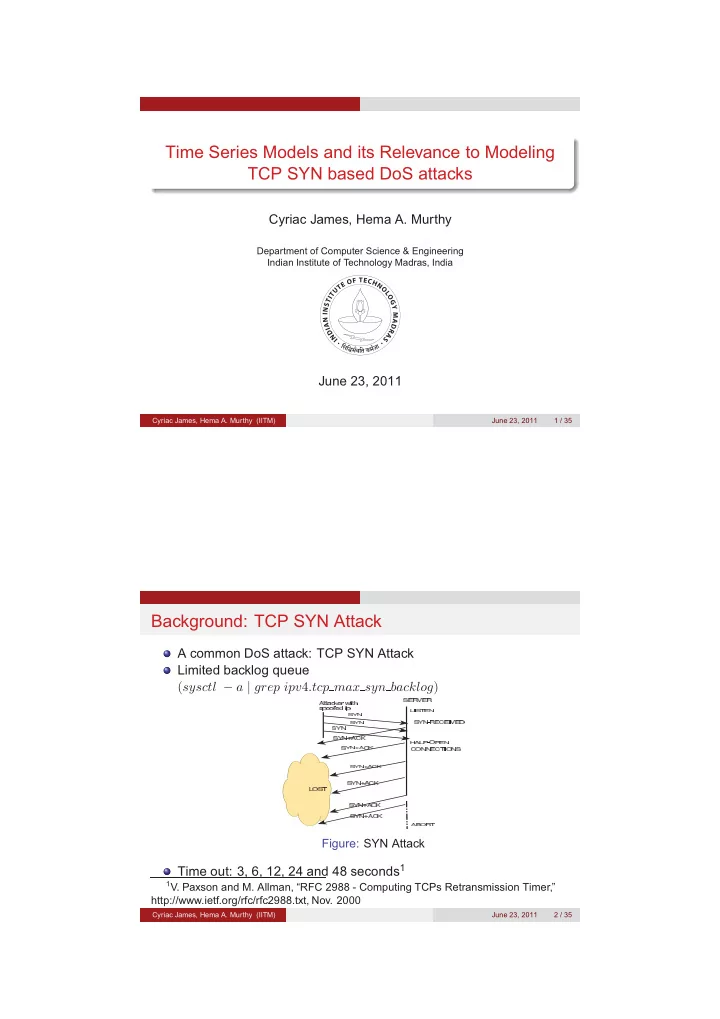
A common DoS attack: TCP SYN Attack Limited backlog queue (sysctl − a | grep ipv4.tcp max syn backlog)

Figure: SYN Attack

Time out: 3, 6, 12, 24 and 48 seconds1

• 1V. Paxson and M. Allman, “RFC 2988 - Computing TCPs Retransmission Timer,”

http://www.ietf.org/rfc/rfc2988.txt, Nov. 2000

Cyriac James, Hema A. Murthy (IITM) June 23, 2011 2 / 35

Outline

Related Work Motivation for the Work Network Trace Representing Network Traffic as a Discrete Time Signal Time Series Models Analysis and Results Conclusion

Cyriac James, Hema A. Murthy (IITM) June 23, 2011 3 / 35

Related Work

Popular statistical work based on CUSUM algorithm by H. Wang et al - for the edge routers

SYN - FIN 1 SYN - SYN/ACK 2

Drawbacks

Series assumed to be i.i.d

Traffic burstiness and non-stationarity: Local-Area Network3 and Wide-Area Network 4

• 1H. Wang, D. Zhang, and K. G. Shin, “Detecting syn flooding attacks,“ Proceedings
• f the IEEE INFOCOM, 2002
• 2H. Wang, D. Zhang, and K. Shin, ”Syn-dog: Sniffing syn flooding sources,” ICDCS,

2002

• 3W. E. Leland, M. S. Taqqu, W. Willinger, and D. V. Wilson, “On the self-similar

nature of ethernet traffic,” in IEEE/ACM Transactions on Networking, 1994

• 4V. Paxson and S. Floyd, “Wide-Area Traffic: The Failure of Poisson Modeling,“ in

IEEE/ACM Transactions on Networking, 1995

Cyriac James, Hema A. Murthy (IITM) June 23, 2011 4 / 35

Related Work

Later, there were quite a few work based on Box-Jenkins Time Series Models - solution at the victim server Modeling the outstanding TCP requests1 Modeling the service rate2 Based on modeling the flow level features3 Modeling the web traffic4

• 1D. M. Divakaran, H. A. Murthy, and T. A. Gonsalves, ”Detection of SYN flooding

attacks using linear prediction analysis,“ ICON, 2006

• 2G. Zhang, S. Jiang, G. Wei, and Q. Guan, ”A prediction-based detection algorithm

against distributed denial-of-service attacks,“ in Proceedings of IWCMC, 2009

• 3J. Cheng, J. Yin, C. Wu, B. Zhang, and Y. Liu, ”DDoS attack detection method

based on linear prediction model,“ in ICIC, 2009

• 4W. U. Qing-tao and S. Zhi-qing, ”Detecting DD O S attacks against web server

using time series analysis,“ Wuhan Univesity Journal of Natural Sciences, vol. 11, no. 1, pp. 175-180, 2006

Cyriac James, Hema A. Murthy (IITM) June 23, 2011 5 / 35

Motivation for the Work

Some of the major drawbacks of these work are: Assumptions of time invariance and stability of the process

Window sizes of the order of seconds or lesser Can we have a model valid for a longer period?

Lacks description on:

Model identification Model validation

Relevance of linear time series models?

Cyriac James, Hema A. Murthy (IITM) June 23, 2011 6 / 35

Network Trace

Figure: Tenet Network Architecture

Traces collected at the edge router using tcpdump Feature: SYN - SYN/ACK, also called half-open count Sampling Interval: 10 seconds

Data Set-1: 26th July 2010 to 30th July 2010 Data Set-2: 23rd August 2010 to 27th August 2010 Data Set-3: 20th September 2010 to 24th September 2010

Cyriac James, Hema A. Murthy (IITM) June 23, 2011 7 / 35 Representing Network Traffic as a Discrete Time Signal

Representing Network Traffic as a Discrete Time Signal

Cyriac James, Hema A. Murthy (IITM) June 23, 2011 8 / 35

Representing Network Traffic as a Discrete Time Signal

Discrete Time Signal

2 4 6 8 10 12 14 16 18 20 2 4 6 8 10 12 14 16 18 Time Amplitude Discrete Signal

Figure: Network Signal

No access to input signals Consider the series as a sequence of impulse responses µt, for time t ≥ 0

Cyriac James, Hema A. Murthy (IITM) June 23, 2011 9 / 35 Representing Network Traffic as a Discrete Time Signal

Stability of the System

For a linear system, Total Response = Zero-State Response + Zero-Input Response1 External Stability: Zero-State Response Internal Stability: Zero-Input Response Internal Stability ⇒ External Stability1 For internal stability, Impulse response must die-off

∞

• j=0

|µj| < ∞ (1) µj: Impulse response at jth time lag

• 1B. P

. Lathi. “Principles of Linear Systems and Signals”, Oxford University Press, 2009 Cyriac James, Hema A. Murthy (IITM) June 23, 2011 10 / 35

Time Series Models

Box-Jenkins Time Series Models

Cyriac James, Hema A. Murthy (IITM) June 23, 2011 11 / 35 Time Series Models

Time Series Models

Idea from the observations of Yule 1 xt = at + α1at−1 + α2at−2 + ... (2) xt: Output Signal at time t at, at−1, ...: Random shocks or white noise process α1, α2...: Model coefficients Also called Linear Filter Model Stationarity: First and Second order moments finite and independent of time2 LTI and Stability ⇔ Stationarity Can be used to build models for prediction

• 1G. U. Yule, “On a method of investigating periodicities in distributed series, with special reference to Wolfer’s sunspot

numbers”, Philos. Trans. Roy. Soc. A226, 267-298, 1927

• 2G. E. P

. Box, G. M. Jenkins, and G. C. Reinsel. “Time Series Analysis: Forecasting and Control”, Pearson Education, 1994 Cyriac James, Hema A. Murthy (IITM) June 23, 2011 12 / 35

Time Series Models

Auto-Regressive(AR) Model

An AR model can be written as xt = α1xt−1 + α2xt−2 + .... + αpxt−p + at (3) xt,xt−1, ...: Output values α1, α2, ...: Model coefficients, where p is the model order at: Random shock at time t Can be written as an infinite series of random shocks Consider an AR(2) model: xt = α1xt−1 + α2xt−2 + at (4) xt−1 = α1xt−2 + α2xt−3 + at−1 (5) xt−2 = α1xt−3 + α2xt−4 + at−2 (6) . . . xt = at + ψ1at−1 + ψ2at−2 + ..... (7)

Cyriac James, Hema A. Murthy (IITM) June 23, 2011 13 / 35 Time Series Models

Auto-Regressive(AR) Model

Computing ACF: E(xtxt−k) = E(atxt−k + ψ1at−1xt−k + ψ2at−2xt−k + .....) (8) γk = E(xt−kat−1) + ψ1E(xt−kat−1) + ψ2E(xt−kat−2) + .... (9) where γK is the autocovariance. Above equation can be generalised into: γk = σ2

a ∞

• j=0

ψjψj+k (10) σ2

a: Variance of at with mean zero

In terms of the impulse response (ACF), it becomes ρk = σ2

a

∞

j=0 ψjψj+k

γ0 (11) Hence, an AR process is an infinite impulse response system For stability ⇒ ∞

j=0 |ψj| < ∞

Cyriac James, Hema A. Murthy (IITM) June 23, 2011 14 / 35

Time Series Models

Auto-Regressive(AR) Model

Multiply with xt−k on Equation (4) and take expectation on both sides: γk = α1γk−1 + α2γk−2 (12) Dividing by γ0, (12) becomes: ρk = α1ρk−1 + α2ρk−2 (13) ρk − α1ρk−1 − α2ρk−2 = 0 (14) Characteristic equation: λ2 − α1λ − α2 = 0 (15) The general solution is of the form: ρk = C1(λ1)k + C2(λ2)k (16) λ1, λ2: Roots (if distinct) C1 and C2: Arbitary constants For Stability ⇒ |λ1| < 1 and |λ2| < 1 Yule-Walker Equation - Estimating model coefficients

Cyriac James, Hema A. Murthy (IITM) June 23, 2011 15 / 35 Time Series Models

Moving Average(MA) Model

An MA model can be written as xt = at − ψ1at−1 − ψ2at−2 − ... − ψ2at−q (17) xt: Output Signal at time t at, at−1, ...: Random shocks or white noise process ψ1, ψ2..., ψq: Model coefficients, where q is the model order Finite linear filter model Can be written as an infinite series of past values Consider an MA model of order 1 xt = at − ψ1at−1 (18)

Cyriac James, Hema A. Murthy (IITM) June 23, 2011 16 / 35

Time Series Models

Moving Average(MA) Model

Multiply with xt−k on equation (18) and take expectation on both sides, γk = E(atxt−k − ψ1at−1xt−k)γ0 = E(atxt − ψ1at−1xt) (19) γ0 = E(at(at − ψ1at−1) − ψ1at−1(at − ψ1at−1) (20) γ0 = σ2

a + ψ2 1σ2 a

(21) γ1 = −ψ1σ2

a

(22) γ2 = 0 (23) γk = 0 for all values of k > 1 Hence, an MA process is a finite impulse response system Time invariant MA process is always stationary

Cyriac James, Hema A. Murthy (IITM) June 23, 2011 17 / 35 Time Series Models

Duality Property: For Model Identification

For an AR(p) process, ACF converges slowly, but PACF cut-off after lag p For an MA(q) process, PACF converges slowly, but ACF cut-off after lag q

Cyriac James, Hema A. Murthy (IITM) June 23, 2011 18 / 35

Time Series Models

Time Series Transformations

Study on Time invariant feature - inconclusive Transformation of Time Series Averaging and Differencing

Cyriac James, Hema A. Murthy (IITM) June 23, 2011 19 / 35 Time Series Models

Average Series

2000 4000 6000 8000 50 100 150 200 250 300 350 Sampling Interval (Seconds) Average half open count Data Set−1,Monday 2000 4000 6000 8000 50 100 150 200 250 300 350 Sampling Interval (Seconds) Average half open count Data Set−1,Tuesday 2000 4000 6000 8000 50 100 150 200 250 300 350 Sampling Interval (Seconds) Average half open count Data Set−1,Wednesday 2000 4000 6000 8000 50 100 150 200 250 300 350 Sampling Interval (Seconds) Average half open count Data Set−1,Thursday

Figure: Average Time Series

Cyriac James, Hema A. Murthy (IITM) June 23, 2011 20 / 35

Time Series Models

Difference Series

2000 4000 6000 8000 50 100 150 200 250 300 350 Sampling Interval (Seconds) Half open count:First difference Data Set−1,Monday 2000 4000 6000 8000 50 100 150 200 250 300 350 Sampling Interval (Seconds) Half open count:First difference Data Set−1,Tuesday 2000 4000 6000 8000 50 100 150 200 250 300 350 Sampling Interval (Seconds) Half open count:First difference Data Set−1,Wednesday 2000 4000 6000 8000 50 100 150 200 250 300 350 Sampling Interval (Seconds) Half open count:First difference Data Set−1,Thursday

Figure: Difference Time Series

Cyriac James, Hema A. Murthy (IITM) June 23, 2011 21 / 35 Analysis and Results

Analysis and Results

Cyriac James, Hema A. Murthy (IITM) June 23, 2011 22 / 35

Analysis and Results

Stationarity Check: Mean Estimation

Day Data Set-1 Dat Set-2 Data Set-3 Monday 13.4132 7.8968 8.1603 Tuesday 11.4301 8.1568 6.7047 Wednesday 14.0949 8.4121 4.9967 Thursday 14.3704 8.4447 4.7113 Friday 13.3957 8.2669 6.0029 Average 13.3409 8.2355 6.1152

(a) Mean: Original Series

Day Data Set-1 Dat Set-2 Data Set-3 Monday 5.5403 5.0499 4.8475 Tuesday 5.0008 5.0958 4.2121 Wednesday 5.6499 5.1832 3.7834 Thursday 5.7435 5.0452 3.6704 Friday 5.3730 5.2722 3.9951 Average 5.4615 5.1292 4.1017

(b) Mean: Difference Series

Day Data Set-1 Dat Set-2 Data Set-3 Monday 13.4352 7.8969 8.1667 Tuesday 11.4376 8.1533 6.7134 Wednesday 14.1062 8.4100 4.9954 Thursday 14.3830 8.4461 4.7138 Friday 13.3990 8.2724 6.0130 Average 13.3524 8.23572 6.1204

(c) Mean: Average Series

Cyriac James, Hema A. Murthy (IITM) June 23, 2011 23 / 35 Analysis and Results

Stationarity Check: Autocorrelation Estimation of Original Series

2 4 6 8 10 12 14 16 18 20 −0.2 0.2 0.4 0.6 0.8 Lag ACF Data Set − 1 Monday Tuesday Wednesday Thursday Friday Zero Reference

(d) ACF: Data Set-1

2 4 6 8 10 12 14 16 18 20 −0.2 0.2 0.4 0.6 0.8 Lag ACF Data Set − 2 Monday Tuesday Wednesday Thursday Friday Zero Reference

(e) ACF: Data Set-2

2 4 6 8 10 12 14 16 18 20 −0.2 0.2 0.4 0.6 0.8 Lag ACF Data Set − 3 Monday Tuesday Wednesday Thursday Friday Zero Reference

(f) ACF: Data Set-3

Cyriac James, Hema A. Murthy (IITM) June 23, 2011 24 / 35

Analysis and Results

Stationarity Check: Autocorrelation Estimation of Difference Series

2 4 6 8 10 12 14 16 18 20 −0.2 0.2 0.4 0.6 0.8 Lag ACF Data Set − 1 Monday Tuesday Wednesday Thursday Friday Zero Reference

(g) ACF: Data Set-1

2 4 6 8 10 12 14 16 18 20 −0.2 0.2 0.4 0.6 0.8 Lag ACF Data Set − 2 Monday Tuesday Wednesday Thursday Friday Zero Reference

(h) ACF: Data Set-2

2 4 6 8 10 12 14 16 18 20 −0.2 0.2 0.4 0.6 0.8 Lag ACF Data Set − 3 Monday Tuesday Wednesday Thursday Friday Zero Reference

(i) ACF: Data Set-3

Cyriac James, Hema A. Murthy (IITM) June 23, 2011 25 / 35 Analysis and Results

Stationarity Check: Autocorrelation Estimation of Average Series

2 4 6 8 10 12 14 16 18 20 −0.2 0.2 0.4 0.6 0.8

Lag ACF Data Set − 1 Monday Tuesday Wednesday Thursday Friday Zero Reference

(j) ACF: Data Set-1

2 4 6 8 10 12 14 16 18 20 −0.2 0.2 0.4 0.6 0.8 Lag ACF Data Set − 2 Monday Tuesday Wednesday Thursday Friday Zero Reference

(k) ACF: Data Set-2

2 4 6 8 10 12 14 16 18 20 −0.2 0.2 0.4 0.6 0.8 Lag ACF Data Set − 3 Monday Tuesday Wednesday Thursday Friday Zero Reference

(l) ACF: Data Set-3

Cyriac James, Hema A. Murthy (IITM) June 23, 2011 26 / 35

Analysis and Results

Stability Check

−1 −0.5 0.5 1 −1 −0.8 −0.6 −0.4 −0.2 0.2 0.4 0.6 0.8 1 Real Axis Imaginary Axis

(m) Roots: Orig. Series

−1 −0.5 0.5 1 −1 −0.8 −0.6 −0.4 −0.2 0.2 0.4 0.6 0.8 1 Real Axis Imaginary Axis

(n) Roots: Diff. Series

−1 −0.5 0.5 1 −1 −0.5 0.5 1 Real Axis Imaginary Axis

(o) Roots: Avg. Series

Cyriac James, Hema A. Murthy (IITM) June 23, 2011 27 / 35 Analysis and Results

Model Identification

2 4 6 8 10 12 14 16 18 20 −0.2 0.2 0.4 0.6 0.8 Lag Sample Autocorrelation Sample Autocorrelation Function (ACF)

(p) Sample ACF - Difference Series

2 4 6 8 10 12 14 16 18 20 −0.2 0.2 0.4 0.6 0.8 Lag Sample Partial Autocorrelations Sample Partial Autocorrelation Function

(q) Sample PACF - Difference Series

Cyriac James, Hema A. Murthy (IITM) June 23, 2011 28 / 35

Analysis and Results

Modeling and Prediction

Only AR and no MA component AR model of order 2 - from PACF Parameter Estimation: Yule-Walker Method Training: One day data

Cyriac James, Hema A. Murthy (IITM) June 23, 2011 29 / 35 Analysis and Results

Model Validation: ACF Spread of Prediction Error

Monday Tuesday Wednesday Thursday Friday −0.04 −0.02 0.02 0.04 0.06 0.08 0.1 0.12 ACF Data Set−1 95% Confidence Interval 95% Spread (1.9 Times Inter−Quartile Range)

(r) Data Set-1

Monday Tuesday Wednesday Thursday Friday −0.04 −0.02 0.02 0.04 0.06 0.08 0.1 0.12 ACF Data Set−1 95% Confidence Interval 95% Spread (1.9 Times Inter−Quartile Range)

(s) Data Set-2

Monday Tuesday Wednesday Thursday Friday −0.04 −0.02 0.02 0.04 0.06 0.08 0.1 0.12 ACF Data Set−1 95% Confidence Interval 95% Spread (1.9 Times Inter−Quartile Range)

(t) Data Set-3

Cyriac James, Hema A. Murthy (IITM) June 23, 2011 30 / 35

Analysis and Results

Model Validation: Root Mean Square Error

Day Model Mon-1 Model Mon-2 Model Mon-3 Mon-1 9.0393 9.0493 9.0509 Tue-1 6.6171 6.6318 6.6235 Wed-1 7.5437 7.5765 7.5391 Thur-1 7.6595 7.6819 7.6610 Fri-1 6.2821 6.3041 6.2892 Mon-2 7.6121 7.6061 7.6297 Tue-2 7.7220 7.7161 7.7566 Wed-2 13.3783 13.4851 13.3488 Thur-2 7.5915 7.5793 7.6356 Fri-2 7.7785 7.7825 7.7899 Mon-3 7.6859 7.7005 7.6736 Tue-3 6.4507 6.4603 6.4648 Wed-3 7.5276 7.5402 7.5327 Thur-3 6.9074 6.8949 6.9275 Fri-3 8.1178 8.1250 8.1197

Figure: RMSE: Model built on Monday Traffic

Cyriac James, Hema A. Murthy (IITM) June 23, 2011 31 / 35 Analysis and Results

Model Validation: N-fold Cross Validation

1 2 3 4 5 6 7 8 9 10 11 12 13 14 15 −4 −2 2 4 6 8 10 12 Days Prediction Error N−Fold Cross Validation Mon−1 Tue−1 Wed−1 Thur−1 Fri−1 Mon−2 Tue−2 Wed−2 Thur−2 Fri−2 Mon−3 Tue−3 Wed−3 Thur−3 Fri−3 Outlier (Wednesday, Data Set−2)

Mean and Variance consistent across all models Model valid for a long period of time Gives an estimate of threshold to be fixed

Cyriac James, Hema A. Murthy (IITM) June 23, 2011 32 / 35

Analysis and Results

Prediction of SYN Attack

Trace driven Simulation Results are ensemble average over 50 such simulated attacks SYN rate: 10 syn/sec to 20 syn/sec Threshold error based on RMSE

50 100 150 200 250 300 350 400 450 500 50 100 150 200 Data Set − 1 Sampling Interval (in seconds) Prediction Error Attack Period Possible False Alarms

Cyriac James, Hema A. Murthy (IITM) June 23, 2011 33 / 35 Analysis and Results

Detection Efficacy

2 3 4 5 6 7 8 9 10 0.1 0.2 0.3 0.4 0.5 0.6 0.7 Threshold Probability Probability of False Postive (FP) Probability of False Negative (FN) Threshold value for 0% FN and 11% FP

(a) False Positive Vs False Negative

2 3 4 5 6 7 8 9 10 50 100 150 200 Threshold Detection Delay (in seconds)

(b) Detection Delay

Cyriac James, Hema A. Murthy (IITM) June 23, 2011 34 / 35

Analysis and Results

Conclusion

Systematic approach

Stationarity Stability Appropriate Transformation

Stressed on model identification and validation Demonstrated the efficacy of the model

For modeling normal traffic For longer period of time Detecting TCP SYN DoS attacks

Effective for Distributed SYN attacks as well Approach can be extended for other DoS attacks as well

Cyriac James, Hema A. Murthy (IITM) June 23, 2011 35 / 35