
SLIDE 1
Thinking in Frequency
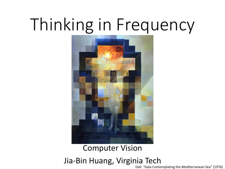
Computer Vision Jia-Bin Huang, Virginia Tech
Dali: “Gala Contemplating the Mediterranean Sea” (1976)
Thinking in Frequency Computer Vision Jia-Bin Huang, Virginia Tech - - PowerPoint PPT Presentation
Thinking in Frequency Computer Vision Jia-Bin Huang, Virginia Tech Dali: Gala Contemplating the Mediterranean Sea (1976) Administrative stuffs HW 0 will be posted on Sunday (Sept 2). Due date: Sept 10 HW 1 will be posted on
Computer Vision Jia-Bin Huang, Virginia Tech
Dali: “Gala Contemplating the Mediterranean Sea” (1976)
product at each position
(among many other uses)
filters
1 1 1 1 1 1 1 1 1
Fill in the blanks:
a) _ = D * B b) A = _ * _ c) F = D * _ d) _ = D * D
A B C D E F G H I Filtering Operator
Slide: Hoiem
Mean abs responses Filters
random occurrences of black and white pixels
drawn from a Gaussian normal distribution
Source: S. Seitz
factors
Source: M. Hebert
Smoothing with larger standard deviations suppresses noise, but also blurs the image
3x3 5x5 7x7
selecting the median intensity in the window
Source: K. Grauman
Source: K. Grauman
Salt-and-pepper noise Median filtered
Source: M. Hebert
3x3 5x5 7x7 Gaussian Median
http://vision.ai.uiuc.edu/?p=1455 Image:
Bilateral filtering
Carlo Tomasi, Roberto Manduchi, Bilateral Filtering for Gray and Color Images, ICCV, 1998.
Original Gaussian Bilateral spatial similarity (e.g., intensity)
product at each position
(among many other uses)
filters
1 1 1 1 1 1 1 1 1
“Hybrid Images,” SIGGRAPH 2006
Slide credit: Derek Hoiem
Why do we get different, distance-dependent interpretations of hybrid images?
Slide credit: Derek Hoiem
Why does a lower resolution image still make sense to us? What do we lose?
Image: http://www.flickr.com/photos/igorms/136916757/ Slide credit: Derek Hoiem
had crazy idea (1807):
Any univariate function can be rewritten as a weighted sum of sines and cosines of different frequencies.
Laplace, Poisson and
English until 1878!
restrictions
...the manner in which the author arrives at these equations is not exempt of difficulties and...his analysis to integrate them still leaves something to be desired on the score of generality and even rigour. Laplace Lagrange Legendre
Slides: Efros
How would math have changed if the Slanket or Snuggie had been invented?
Slide credit: James Hays
Our building block: Add enough of them to get any signal f(x) you want!
= +
Slides: Efros
= + =
= + =
= + =
= + =
= + =
=
1
1 sin(2 )
k
A kt k π
∞ =
different magnitudes
same way
xkcd.com
Cats(?)
http://sharp.bu.edu/~slehar/fourier/fourier.html#filtering
Intensity Image Fourier Image
http://sharp.bu.edu/~slehar/fourier/fourier.html#filtering More: http://www.cs.unm.edu/~brayer/vision/fourier.html
Teases away fast vs. slow changes in the image.
Slide credit: A Efros
Image as a sum of basis images
in Matlab, check out: imagesc(log(abs(fftshift(fft2(im)))));
each frequency
and complex numbers
2 2
) ( ) ( ω ω I R A + ± =
) ( ) ( tan 1 ω ω φ R I
−
=
Amplitude: Euler’s formula: Phase:
Salvador Dali invented Hybrid Images? Salvador Dali “Gala Contemplating the Mediterranean Sea, which at 30 meters becomes the portrait
Log Magnitude Strong Vertical Frequency (Sharp Horizontal Edge) Strong Horz. Frequency (Sharp Vert. Edge) Diagonal Frequencies
Low Frequencies
Continuous Discrete
k = -N/2..N/2
Fast Fourier Transform (FFT): NlogN
the origin
its Fourier transform
See Szeliski Book (3.4)
functions is the product of their Fourier transforms
Fourier transforms is the convolution of the two inverse Fourier transforms
multiplication in frequency domain!
1 1 1
− − −
1
2
1
Spatial domain Frequency domain
FFT FFT
Inverse FFT
im = … % im: gray-scale floating point image [imh, imw] = size(im); fftsize = 1024; % fftsize: should be order of 2 (for speed) and include padding hs = 50; % fil: Gaussian filter fil = fspecial('gaussian', hs*2+1, 10); % im_fft = fft2(im, fftsize, fftsize); % 1) fft im with padding fil_fft = fft2(fil, fftsize, fftsize); % 2) fft fil, pad to same size as image im_fil_fft = im_fft .* fil_fft; % 3) multiply fft images im_fil = ifft2(im_fil_fft); % 4) inverse fft2 im_fil = im_fil(1+hs:size(im,1)+hs, 1+hs:size(im, 2)+hs); % 5) remove padding figure(1), imagesc(log(abs(fftshift(im_fft)))), axis image, colormap jet
Which has more information, the phase or the magnitude? What happens if you take the phase from one image and combine it with the magnitude from another image?
Magnitude Phase Intensity image
FFT
Inverse FFT
Use random
magnitude
Inverse FFT
Use random phase
Why does the Gaussian give a nice smooth image, but the square filter give edgy artifacts?
Gaussian Box filter
Gaussian
Box Filter
Match the spatial domain image to the Fourier magnitude image
1 5 4 A 3 2 C B D E
This image is too big to fit on the screen. How can we reduce it? How to generate a half- sized version?
Throw away every other row and column to create a 1/2 size image
1/4 1/8
Slide by Steve Seitz
1/4 (2x zoom) 1/8 (4x zoom) 1/2
Slide by Steve Seitz
Why does this look so crufty? Aliasing! What do we do?
Source: F. Durand
Source: L. Zhang
Source: S. Marschner
Source: S. Marschner
Source: D. Forsyth
capture the amount of detail in your image
your signal/image
Source: L. Zhang
(See http://www.michaelbach.de/ot/mot_wagonWheel/index.html)
Source: L. Zhang
https://www.youtube.com/watch?v=QOwzkND_ooU
Examples of GOOD sampling
Examples of BAD sampling -> Aliasing
Forsyth and Ponce 2002
G 1/4 G 1/8 Gaussian 1/2
Source: S. Seitz
G 1/4 G 1/8 Gaussian 1/2
Source: S. Seitz
1/4 (2x zoom) 1/8 (4x zoom) 1/2
Source: S. Seitz
Why does a lower resolution image still make sense to us? What do we lose?
Image: http://www.flickr.com/photos/igorms/136916757/
Why do we get different, distance-dependent interpretations of hybrid images?
Hybrid Image Low-passed Image High-passed Image
repeat each row and column 10 times
interpolation”)
Recall how a digital image is formed
image could be generated, at any resolution and scale
1 2 3 4 5
Adapted from: S. Seitz
d = 1 in this example
1 2 3 4 5
d = 1 in this example
Adapted from: S. Seitz
Recall how a digital image is formed
image could be generated, at any resolution and scale
1 2 3 4 5 2.5 1
d = 1 in this example
Adapted from: S. Seitz
“Ideal” reconstruction Nearest-neighbor interpolation Linear interpolation Gaussian reconstruction
Source: B. Curless
Often implemented without cross-correlation
Better filters give better resampled images
performs linear interpolation (tent function) performs bilinear interpolation
Cubic reconstruction filter
Nearest-neighbor interpolation Bilinear interpolation Bicubic interpolation
Original image: x 10
Also used for resampling
images and filtering in the frequency domain
images (N logN vs. N2 for auto-correlation)