Theory of Computer Science May 6, 2020 E1. Complexity Theory: - - PowerPoint PPT Presentation

theory of computer science
SMART_READER_LITE
LIVE PREVIEW

Theory of Computer Science May 6, 2020 E1. Complexity Theory: - - PowerPoint PPT Presentation

Theory of Computer Science May 6, 2020 E1. Complexity Theory: Motivation and Introduction Theory of Computer Science E1.1 Motivation E1. Complexity Theory: Motivation and Introduction E1.2 How to Measure Runtime? Gabriele R oger E1.3


slide-1
SLIDE 1

Theory of Computer Science

  • E1. Complexity Theory: Motivation and Introduction

Gabriele R¨

  • ger

University of Basel

May 6, 2020

Gabriele R¨

  • ger (University of Basel)

Theory of Computer Science May 6, 2020 1 / 38

Theory of Computer Science

May 6, 2020 — E1. Complexity Theory: Motivation and Introduction

E1.1 Motivation E1.2 How to Measure Runtime? E1.3 Decision Problems E1.4 Nondeterminism

Gabriele R¨

  • ger (University of Basel)

Theory of Computer Science May 6, 2020 2 / 38

Overview: Course

contents of this course:

  • A. background

⊲ mathematical foundations and proof techniques

  • B. logic

⊲ How can knowledge be represented? ⊲ How can reasoning be automated?

  • C. automata theory and formal languages

⊲ What is a computation?

  • D. Turing computability

⊲ What can be computed at all?

  • E. complexity theory

⊲ What can be computed efficiently?

  • F. more computability theory

⊲ Other models of computability

Gabriele R¨

  • ger (University of Basel)

Theory of Computer Science May 6, 2020 3 / 38
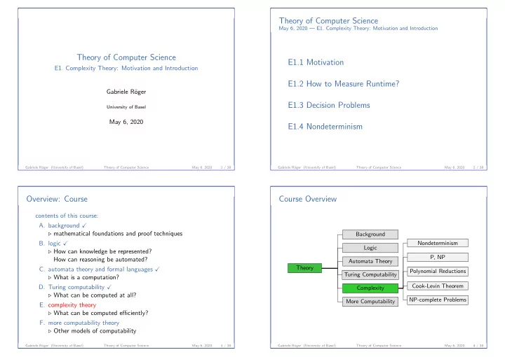
Course Overview

Theory Background Logic Automata Theory Turing Computability Complexity Nondeterminism P, NP Polynomial Reductions Cook-Levin Theorem NP-complete Problems More Computability

Gabriele R¨

  • ger (University of Basel)

Theory of Computer Science May 6, 2020 4 / 38

slide-2
SLIDE 2
  • E1. Complexity Theory: Motivation and Introduction

Motivation

E1.1 Motivation

Gabriele R¨

  • ger (University of Basel)

Theory of Computer Science May 6, 2020 5 / 38

  • E1. Complexity Theory: Motivation and Introduction

Motivation

A Scenario (1)

Example Scenario ◮ You are a programmer at a logistics company. ◮ Your boss gives you the task of developing a program to optimize the route of a delivery truck:

◮ The truck begins its route at the company depot. ◮ It has to visit 50 stops. ◮ You know the distances between all relevant locations (stops and depot). ◮ Your program should compute a tour visiting all stops and returning to the depot on a shortest route.

Gabriele R¨

  • ger (University of Basel)

Theory of Computer Science May 6, 2020 6 / 38

  • E1. Complexity Theory: Motivation and Introduction

Motivation

A Scenario (2)

Example Scenario (ctd.) ◮ You work on the problem for weeks, but you do not manage to complete the task. ◮ All of your attempted programs

◮ compute routes that are possibly suboptimal, or ◮ do not terminate in reasonable time (say: within a month).

◮ What do you say to your boss?

Gabriele R¨

  • ger (University of Basel)

Theory of Computer Science May 6, 2020 7 / 38

  • E1. Complexity Theory: Motivation and Introduction

Motivation

What You Don’t Want to Say

“I can’t find an efficient algorithm, I guess I’m just too dumb.”

Source: M. Garey & D. Johnson, Computers and Intractability, Freeman 1979, p. 2 Gabriele R¨

  • ger (University of Basel)

Theory of Computer Science May 6, 2020 8 / 38

slide-3
SLIDE 3
  • E1. Complexity Theory: Motivation and Introduction

Motivation

What You Would Like to Say

“I can’t find an efficient algorithm, because no such algorithm is possible!”

Source: M. Garey & D. Johnson, Computers and Intractability, Freeman 1979, p. 2 Gabriele R¨

  • ger (University of Basel)

Theory of Computer Science May 6, 2020 9 / 38

  • E1. Complexity Theory: Motivation and Introduction

Motivation

What Complexity Theory Allows You to Say

“I can’t find an efficient algorithm, but neither can all these famous people.”

Source: M. Garey & D. Johnson, Computers and Intractability, Freeman 1979, p. 3 Gabriele R¨

  • ger (University of Basel)

Theory of Computer Science May 6, 2020 10 / 38

  • E1. Complexity Theory: Motivation and Introduction

Motivation

Why Complexity Theory?

Complexity Theory Complexity theory tells us which problems can be solved quickly (“simple problems”) and which ones cannot (“hard problems”).

German: Komplexit¨ atstheorie

◮ This is useful in practice because simple and hard problems require different techniques to solve. ◮ If we can show that a problem is hard we do not need to waste

  • ur time with the (futile) search for a “simple” algorithm.

Gabriele R¨

  • ger (University of Basel)

Theory of Computer Science May 6, 2020 11 / 38

  • E1. Complexity Theory: Motivation and Introduction

Motivation

Why Reductions?

Reductions An important part of complexity theory are (polynomial) reductions that show how a given problem P can be reduced to another problem Q.

German: Reduktionen

◮ useful for theoretical analysis of P and Q because it allows us to transfer our knowledge between them ◮ often also useful for practical algorithms for P: reduce P to Q and then use the best known algorithm for Q

Gabriele R¨

  • ger (University of Basel)

Theory of Computer Science May 6, 2020 12 / 38

slide-4
SLIDE 4
  • E1. Complexity Theory: Motivation and Introduction

Motivation

Test Your Intuition! (1)

◮ The following slide lists some graph problems. ◮ The input is always a directed graph G = V , E. ◮ How difficult are the problems in your opinion? ◮ Sort the problems from easiest (= requires least amount of time to solve) to hardest (= requires most time to solve) ◮ no justification necessary, just follow your intuition! ◮ anonymous and not graded

Gabriele R¨

  • ger (University of Basel)

Theory of Computer Science May 6, 2020 13 / 38

  • E1. Complexity Theory: Motivation and Introduction

Motivation

Test Your Intuition! (2)

1 Find a simple path (= without cycle)

from u ∈ V to v ∈ V with minimal length.

2 Find a simple path (= without cycle)

from u ∈ V to v ∈ V with maximal length.

3 Determine whether G is strongly connected

(every node is reachable from every other node).

4 Find a cycle (non-empty path from u to u for any u ∈ V ;

multiple visits of nodes are allowed).

5 Find a cycle that visits all nodes. 6 Find a cycle that visits a given node u. 7 Find a path that visits all nodes without repeating a node. 8 Find a path that uses all edges without repeating an edge. Gabriele R¨

  • ger (University of Basel)

Theory of Computer Science May 6, 2020 14 / 38

  • E1. Complexity Theory: Motivation and Introduction

How to Measure Runtime?

E1.2 How to Measure Runtime?

Gabriele R¨

  • ger (University of Basel)

Theory of Computer Science May 6, 2020 15 / 38

  • E1. Complexity Theory: Motivation and Introduction

How to Measure Runtime?

How to Measure Runtime?

◮ Time complexity is a way to measure how much time it takes to solve a problem. ◮ How can we define such a measure appropriately?

German: Zeitkomplexit¨ at/Zeitaufwand

Gabriele R¨

  • ger (University of Basel)

Theory of Computer Science May 6, 2020 16 / 38

slide-5
SLIDE 5
  • E1. Complexity Theory: Motivation and Introduction

How to Measure Runtime?

Example Statements about Runtime

Example statements about runtime: ◮ “Running sort /usr/share/dict/words

  • n the computer dakar takes 0.035 seconds.”

◮ “With a 1 MiB input file, sort takes at most 1 second on a modern computer.” ◮ “Quicksort is faster than sorting by insertion.” ◮ “Sorting by insertion is slow.” Very different statements with different pros and cons.

Gabriele R¨

  • ger (University of Basel)

Theory of Computer Science May 6, 2020 17 / 38

  • E1. Complexity Theory: Motivation and Introduction

How to Measure Runtime?

Precise Statements vs. General Statements

Example Statement about Runtime “Running sort /usr/share/dict/words

  • n the computer dakar takes 0.035 seconds.”

advantage: very precise disadvantage: not general ◮ input-specific: What if we want to sort other files? ◮ machine-specific: What happens on a different computer? ◮ even situation-specific: Will we get the same result tomorrow that we got today?

Gabriele R¨

  • ger (University of Basel)

Theory of Computer Science May 6, 2020 18 / 38

  • E1. Complexity Theory: Motivation and Introduction

How to Measure Runtime?

General Statements about Runtime

In this course we want to make general statements about runtime. We accomplish this in three ways:

  • 1. General Inputs

Instead of concrete inputs, we talk about general types of input: ◮ Example: runtime to sort an input of size n in the worst case ◮ Example: runtime to sort an input of size n in the average case here: runtime for input size n in the worst case

Gabriele R¨

  • ger (University of Basel)

Theory of Computer Science May 6, 2020 19 / 38

  • E1. Complexity Theory: Motivation and Introduction

How to Measure Runtime?

General Statements about Runtime

In this course we want to make general statements about runtime. We accomplish this in three ways:

  • 2. Ignoring Details

Instead of exact formulas for the runtime we specify the order of magnitude: ◮ Example: instead of saying that we need time ⌈1.2n log n⌉ − 4n + 100, we say that we need time O(n log n). ◮ Example: instead of saying that we need time O(n log n), O(n2) or O(n4), we say that we need polynomial time. here: What can be computed in polynomial time?

Gabriele R¨

  • ger (University of Basel)

Theory of Computer Science May 6, 2020 20 / 38

slide-6
SLIDE 6
  • E1. Complexity Theory: Motivation and Introduction

How to Measure Runtime?

General Statements about Runtime

In this course we want to make general statements about runtime. We accomplish this in three ways:

  • 3. Abstract Cost Measures

Instead of the runtime on a concrete computer we consider a more abstract cost measure: ◮ Example: count the number of executed machine code statements ◮ Example: count the number of executed Java byte code statements ◮ Example: count the number of element comparisons

  • f a sorting algorithms

here: count the computation steps of a Turing machine (polynomially equivalent to other measures)

Gabriele R¨

  • ger (University of Basel)

Theory of Computer Science May 6, 2020 21 / 38

  • E1. Complexity Theory: Motivation and Introduction

Decision Problems

E1.3 Decision Problems

Gabriele R¨

  • ger (University of Basel)

Theory of Computer Science May 6, 2020 22 / 38

  • E1. Complexity Theory: Motivation and Introduction

Decision Problems

Decision Problems

◮ As before, we simplify our investigation by restricting our attention to decision problems. ◮ More complex computational problems can be solved with multiple queries for an appropriately defined decision problem (“playing 20 questions”). ◮ Formally, decision problems are languages (as before), but we use an informal “given”/“question” notation where possible.

Gabriele R¨

  • ger (University of Basel)

Theory of Computer Science May 6, 2020 23 / 38

  • E1. Complexity Theory: Motivation and Introduction

Decision Problems

Example: Decision vs. General Problem (1)

Definition (Hamilton Cycle) Let G = V , E be a (directed or undirected) graph. A Hamilton cycle of G is a sequence of vertices in V , π = v0, . . . , vn, with the following properties: ◮ π is a path: there is an edge from vi to vi+1 for all 0 ≤ i < n ◮ π is a cycle: v0 = vn ◮ π is simple: vi = vj for all i = j with i, j < n ◮ π is Hamiltonian: all nodes of V are included in π

German: Hamiltonkreis/Hamiltonzyklus

Gabriele R¨

  • ger (University of Basel)

Theory of Computer Science May 6, 2020 24 / 38

slide-7
SLIDE 7
  • E1. Complexity Theory: Motivation and Introduction

Decision Problems

Example: Decision vs. General Problem (2)

Example (Hamilton Cycles in Directed Graphs) P: general problem DirHamiltonCycleGen ◮ Input: directed graph G = V , E ◮ Output: a Hamilton cycle of G or a message that none exists D: decision problem DirHamiltonCycle ◮ Given: directed graph G = V , E ◮ Question: Does G contain a Hamilton cycle? These problems are polynomially equivalent: from a polynomial algorithm for one of the problems

  • ne can construct a polynomial algorithm for the other problem.

(Without proof.)

Gabriele R¨

  • ger (University of Basel)

Theory of Computer Science May 6, 2020 25 / 38

  • E1. Complexity Theory: Motivation and Introduction

Decision Problems

Algorithms for Decision Problems

Algorithms for decision problems: ◮ Where possible, we specify algorithms for decision problems in pseudo-code. ◮ Since they are only yes/no questions, we do not have to return a general result. ◮ Instead we use the statements

◮ ACCEPT to accept the given input (“yes” answer) and ◮ REJECT to reject it (“no” answer).

◮ Where we must be more formal, we use Turing machines and the notion of accepting from chapter C7.

Gabriele R¨

  • ger (University of Basel)

Theory of Computer Science May 6, 2020 26 / 38

  • E1. Complexity Theory: Motivation and Introduction

Nondeterminism

E1.4 Nondeterminism

Gabriele R¨

  • ger (University of Basel)

Theory of Computer Science May 6, 2020 27 / 38

  • E1. Complexity Theory: Motivation and Introduction

Nondeterminism

Course Overview

Theory Background Logic Automata Theory Turing Computability Complexity Nondeterminism P, NP Polynomial Reductions Cook-Levin Theorem NP-complete Problems More Computability

Gabriele R¨

  • ger (University of Basel)

Theory of Computer Science May 6, 2020 28 / 38

slide-8
SLIDE 8
  • E1. Complexity Theory: Motivation and Introduction

Nondeterminism

Nondeterminism

◮ To develop complexity theory, we need the algorithmic concept of nondeterminism. ◮ already known for Turing machines ( chapter C7):

◮ An NTM can have more than one possible successor configuration for a given configuration. ◮ Input x is accepted if there is at least one possible computation (configuration sequence) that leads to an end state.

◮ Here we analogously introduce nondeterminism for pseudo-code.

German: Nichtdeterminismus

Gabriele R¨

  • ger (University of Basel)

Theory of Computer Science May 6, 2020 29 / 38

  • E1. Complexity Theory: Motivation and Introduction

Nondeterminism

Nondeterministic Algorithms

nondeterministic algorithms: ◮ All constructs of deterministic algorithms are also allowed in nondeterministic algorithms: IF, WHILE, etc. ◮ Additionally, there is a nondeterministic assignment: GUESS xi ∈ {0, 1} where xi is a program variable.

German: nichtdeterministische Zuweisung

Gabriele R¨

  • ger (University of Basel)

Theory of Computer Science May 6, 2020 30 / 38

  • E1. Complexity Theory: Motivation and Introduction

Nondeterminism

Nondeterministic Algorithms: Acceptance

◮ Meaning of GUESS xi ∈ {0, 1}: xi is assigned either the value 0 or the value 1. ◮ This implies that the behavior of the program

  • n a given input is no longer uniquely defined:

there are multiple possible execution paths. ◮ The program accepts a given input if at least one execution path leads to an ACCEPT statement. ◮ Otherwise, the input is rejected. Note: asymmetry between accepting and rejecting! (cf. semi-decidability)

Gabriele R¨

  • ger (University of Basel)

Theory of Computer Science May 6, 2020 31 / 38

  • E1. Complexity Theory: Motivation and Introduction

Nondeterminism

More Complex GUESS Statements

◮ We will also guess more than one bit at a time: GUESS x ∈ {1, 2, . . . , n}

  • r more generally

GUESS x ∈ S for a set S. ◮ These are abbreviations and can be split into ⌈log2 n⌉ (or ⌈log2 |S|⌉) “atomic” GUESS statements.

Gabriele R¨

  • ger (University of Basel)

Theory of Computer Science May 6, 2020 32 / 38

slide-9
SLIDE 9
  • E1. Complexity Theory: Motivation and Introduction

Nondeterminism

Example: Nondeterministic Algorithms (1)

Example (DirHamiltonCycle) input: directed graph G = V , E start := an arbitrary node from V current := start remaining := V \ {start} WHILE remaining = ∅: GUESS next ∈ remaining IF current, next / ∈ E: REJECT remaining := remaining \ {next} current := next IF current, start ∈ E: ACCEPT ELSE: REJECT

Gabriele R¨

  • ger (University of Basel)

Theory of Computer Science May 6, 2020 33 / 38

  • E1. Complexity Theory: Motivation and Introduction

Nondeterminism

Example: Nondeterministic Algorithms (2)

◮ With appropriate data structures, this algorithm solves the problem in O(n log n) program steps, where n = |V | + |E| is the size of the input. ◮ How many steps would a deterministic algorithm need?

Gabriele R¨

  • ger (University of Basel)

Theory of Computer Science May 6, 2020 34 / 38

  • E1. Complexity Theory: Motivation and Introduction

Nondeterminism

Guess and Check

◮ The DirHamiltonCycle example illustrates a general design principle for nondeterministic algorithms: guess and check ◮ In general, nondeterministic algorithms can solve a problem by first guessing a “solution” and then verifying that it is indeed a solution. (In the example, these two steps are interleaved.) ◮ If solutions to a problem can be efficiently verified, then the problem can also be efficiently solved if nondeterminism may be used.

German: Raten und Pr¨ ufen

Gabriele R¨

  • ger (University of Basel)

Theory of Computer Science May 6, 2020 35 / 38

  • E1. Complexity Theory: Motivation and Introduction

Nondeterminism

The Power of Nondeterminism

◮ Nondeterministic algorithms are very powerful because they can “guess” the “correct” computation step. ◮ Or, interpreted differently: they go through many possible computations “in parallel”, and it suffices if one of them is successful. ◮ Can they solve problems efficiently (in polynomial time) which deterministic algorithms cannot solve efficiently? ◮ This is the big question!

Gabriele R¨

  • ger (University of Basel)

Theory of Computer Science May 6, 2020 36 / 38

slide-10
SLIDE 10
  • E1. Complexity Theory: Motivation and Introduction

Summary

Summary (1)

◮ Complexity theory deals with the question which problems can be solved efficiently and which ones cannot. ◮ here: focus on what can be computed in polynomial time ◮ To formalize this, we use Turing machines, but other formalisms are polynomially equivalent. ◮ We consider decision problems, but the results directly transfer to general computational problems.

Gabriele R¨

  • ger (University of Basel)

Theory of Computer Science May 6, 2020 37 / 38

  • E1. Complexity Theory: Motivation and Introduction

Summary

Summary (2)

important concept: nondeterminism ◮ Nondeterministic algorithms can “guess”,

  • i. e., perform multiple computations “at the same time”.

◮ An input receives a “yes” answer if at least one computation path accepts it. ◮ in NTMs: with nondeterministic transitions (δ(q, a) contains multiple elements) ◮ in pseudo-code: with GUESS statements

Gabriele R¨

  • ger (University of Basel)

Theory of Computer Science May 6, 2020 38 / 38