The story of the film so far... C.r.v.s X and Y have a joint density - - PowerPoint PPT Presentation

SLIDE 1

Mathematics for Informatics 4a

Jos´ e Figueroa-O’Farrill Lecture 13 7 March 2012

Jos´ e Figueroa-O’Farrill mi4a (Probability) Lecture 13 1 / 21

The story of the film so far...

C.r.v.s X and Y have a joint density f(x, y) with

P((X, Y) ∈ C) =

• C

f(x, y)dx dy

and a joint distribution

F(x, y) = P(X x, Y y) = x

−∞

y

−∞

f(u, v)du dv

with f(x, y) =

∂2 ∂x∂yF(x, y)

X and Y independent iff f(x, y) = fX(x)fY(y)

Geometric probability is fun! (Buffon’s needle) We can calculate the c.d.f. and p.d.f. of Z = g(X, Y)

X, Y independent: fX+Y = fX ⋆ fY (convolution)

Jos´ e Figueroa-O’Farrill mi4a (Probability) Lecture 13 2 / 21

Convolution

Definition Let f, g : R → R be two functions. Their convolution

f ⋆ g : R → R is the function defined by (f ⋆ g)(z) = ∞

−∞

f(x)g(z − x)dx (provided the integral exists)

Properties of the convolution

f ⋆ g = g ⋆ f (f ⋆ g) ⋆ h = f ⋆ (g ⋆ h) (hence we can just write f ⋆ g ⋆ h) f ⋆ g is “smoother” than f or g

Jos´ e Figueroa-O’Farrill mi4a (Probability) Lecture 13 3 / 21

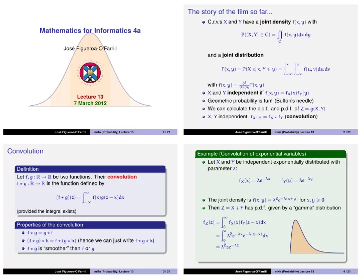
Example (Convolution of exponential variables) Let X and Y be independent exponentially distributed with parameter λ:

fX(x) = λe−λx fY(y) = λe−λy

The joint density is f(x, y) = λ2e−λ(x+y) for x, y 0 Then Z = X + Y has p.d.f. given by a “gamma” distribution

fZ(z) = ∞ fX(x)fY(z − x)dx = z λ2e−λxe−λ(z−x)dx = λ2ze−λz

Jos´ e Figueroa-O’Farrill mi4a (Probability) Lecture 13 4 / 21

SLIDE 2

Example (Independent standard normal random variables)

X, Y: independent, standard normally distributed. Their

sum Z = X + Y has p.d.f.

fZ(z) = ∞

−∞

1 2πe−x2/2e−(z−x)2/2dx

= e−z2/4

2π

∞

−∞

e−(x−z/2)2dx

(complete the square)

= e−z2/4

2π

∞

−∞

e−u2du

(u = x − 1

2z)

=

1 2√πe−z2/4 so it is normally distributed with zero mean and variance 2. More generally, if X has mean µX and variance σ2

X and Y

has mean µY and variance σ2

Y, Z is normally distributed

with mean µX + µY and variance σ2

X + σ2 Y

Jos´ e Figueroa-O’Farrill mi4a (Probability) Lecture 13 5 / 21

Expectations of functions of random variables

Let X and Y be c.r.v.s with joint density f(x, y) Let Z = g(X, Y) for some g : R2 → R The expectation value of Z is defined by

E(Z) =

• g(x, y)f(x, y)dx dy

(provided the integral exists)

We already saw that

E(X + Y) = E(X) + E(Y)

even if X and Y are not independent

Jos´ e Figueroa-O’Farrill mi4a (Probability) Lecture 13 6 / 21

Example (Normally distributed darts) A dart hits a plane target at the point with coordinates (X, Y) where X and Y have joint density

f(x, y) = 1

2πe−(x2+y2)/2 Let R =

• X2 + Y2 be the distance from the bullseye. What is

E(R)? E(R) =

1 2πre−r2/2rdr dθ

= ∞ r2e−r2/2dr = 1

2

∞

−∞

r2e−r2/2dr =

• π

2

∞

−∞

1

√

2π

r2e−r2/2dr =

• π

2

Jos´ e Figueroa-O’Farrill mi4a (Probability) Lecture 13 7 / 21

Example (Normally distributed darts — continued) What is E(R2)?

E(R2) = E(X2 + Y2) = E(X2) + E(Y2) = 1 + 1 = 2

where we used linearity of E, and the fact that E(X2) = Var(X) = 1 and similarly for Y This shows that Var(R) = E(R2) − E(R)2 = 2 − π

2 .

Jos´ e Figueroa-O’Farrill mi4a (Probability) Lecture 13 8 / 21

SLIDE 3

Independent random variables I

Theorem Let X, Y be independent continuous random variables. Then

E(XY) = E(X)E(Y)

Proof.

E(XY) =

• xyf(x, y)dx dy

=

• xyfX(x)fY(y)dx dy

(independence)

=

• xfX(x)dx

yfY(y)dy

• = E(X)E(Y)

Jos´ e Figueroa-O’Farrill mi4a (Probability) Lecture 13 9 / 21

Independent random variables II

As with discrete random variables, we have the following Corollary Let X, Y be independent continuous random variables. Then Var(X + Y) = Var(X) + Var(Y) Definition The covariance and correlation of X and Y are Cov(X, Y) = E(XY) − E(X)E(Y)

ρ(X, Y) =

Cov(X, Y)

• Var(X) Var(Y)

Jos´ e Figueroa-O’Farrill mi4a (Probability) Lecture 13 10 / 21

Example Consider X, Y uniformly distributed on the unit disk D, so that

f(x, y) = 1 π

Then by symmetric integration,

E(XY) = E(X) = E(Y) = 0 = ⇒

Cov(X, Y) = 0 Therefore X, Y are uncorrelated but not independent.

Jos´ e Figueroa-O’Farrill mi4a (Probability) Lecture 13 11 / 21

Example (Continued) On the other hand, U = |X| and V = |Y| are correlated.

E(U) =

• D

|x|1 πdx dy = 2

π

π

2

− π

2

1 r2 cos θdr dθ = 2

π

π

2

− π

2

cos θdθ

1 r2dr = 2

π × 2 × 1 3

=

4 3π

x y

And by symmetry, also E(V) =

4 3π.

Jos´ e Figueroa-O’Farrill mi4a (Probability) Lecture 13 12 / 21

SLIDE 4

Example (Continued) Finally,

E(UV) =

• D

|xy|1 πdx dy = 4

π

π

2

1 r3 sin θ cos θdr dθ = 4

π

π

2

sin θ cos θdθ

1 r3dr = 4

π × 1 2 × 1 4 = 1 2π

x y

Hence

E(UV) − E(U)E(V) =

1 2π − 16 9π2 = 9π−32 18π2 < 0

Jos´ e Figueroa-O’Farrill mi4a (Probability) Lecture 13 13 / 21

Moment generating function of a sum

Let X, Y be independent continuous random variables and let

Z = X + Y. Then MZ(t) = E(etZ) =

• etzfZ(z)dz

=

• etz
• fX(x)fY(z − x)dx dz

=

• et(z−x)etxfX(x)fY(z − x)dx dz

=

• etxfX(x)dx
• etyfY(y)dy

(y = z − x)

= MX(t)MY(t)

Jos´ e Figueroa-O’Farrill mi4a (Probability) Lecture 13 14 / 21

Markov’s inequality

Theorem (Markov’s inequality) Let X be a c.r.v. Then for all ε > 0

P(|X| ε) E(|X|) ε

. Proof.

E(|X|) = ∞

−∞

|x|f(x)dx = −ε

−∞

|x|f(x)dx + ε

−ε

|x|f(x)dx + ∞

ε

|x|f(x)dx ε −ε

−∞

f(x)dx + ε ∞

ε

f(x)dx = εP(|X| ε)

Jos´ e Figueroa-O’Farrill mi4a (Probability) Lecture 13 15 / 21

Chebyshev’s inequality

Theorem (Chebyshev’s inequality) Let X be a c.r.v. with finite mean and variance. Then

P(|X| ε) E(X2) ε2

for all ε > 0 Proof.

E(X2) = ∞

−∞

x2f(x)dx = −ε

−∞

x2f(x)dx + ε

−ε

x2f(x)dx + ∞

ε

x2f(x)dx ε2 −ε

−∞

f(x)dx + ε2 ∞

ε

f(x)dx = ε2P(|X| ε)

Jos´ e Figueroa-O’Farrill mi4a (Probability) Lecture 13 16 / 21

SLIDE 5

Two corollaries of Chebyshev’s inequality

Corollary Let X be a c.r.v. with mean µ and variance σ2. Then for any

ε > 0, P(|X − µ| ε) σ2 ε2

Corollary (The (weak) law of large numbers) Let X1, X2, . . . be i.i.d. continuous random variables with mean

µ and variance σ2 and let Zn = 1

n(X1 + · · · + Xn). Then

∀ε > 0 P(|Zn − µ| < ε) → 1

as n → ∞

Jos´ e Figueroa-O’Farrill mi4a (Probability) Lecture 13 17 / 21

The Chernoff bound

Corollary Let X be a c.r.v. with moment generating function MX(t). Then for any t > 0,

P(X α) e−tαMX(t)

Proof.

P(X α) = P( tX

2 tα 2 ) = P(etX/2 etα/2)

and by Chebyshev’s inequality for etX/2,

P(etX/2 etα/2) E(etX) etα = e−tαMX(t) .

Jos´ e Figueroa-O’Farrill mi4a (Probability) Lecture 13 18 / 21

Waiting times and the exponential distribution

If “rare” and “isolated” events can occur at random in the time interval [0, t], then the number of events N(t) in that time interval can be approximated by a Poisson distribution

P(N(t) = n) = e−λt (λt)n n!

. Let us start at t = 0 and let X be the time of the first event; that is, the waiting time. Clearly, X > t if and only if N(t) = 0, whence

P(X > t) = P(N(t) = 0) = e−λt = ⇒ P(X t) = 1 − e−λt

and differentiating,

fX(t) = λe−λt

whence X is exponentially distributed.

Jos´ e Figueroa-O’Farrill mi4a (Probability) Lecture 13 19 / 21

Example (Radioactivity) The number of radioactive decays in [0, t] is approximated by a Poisson distribution, so decay times are exponentially

• distributed. The time t1/2 in which one half of the particles have

decayed is called the half-life. It is a sensible concept because

• f the “lack of memory” of the exponential distribution.

How are the half-life and the parameter in the exponential distribution related? By definition, P(X t1/2) = 1

2, whence

e−λt1/2 = 1

2 =

⇒ λ = log 2 t1/2

The mean of the exponential distribution: 1

λ = t1/2/ log 2 is

called the mean lifetime. e.g.,t1/2(235U) ≈ 700 × 106 yrs; t1/2(14C) = 5, 730 yrs;

t1/2(137Cs) ≈ 30 yrs

Jos´ e Figueroa-O’Farrill mi4a (Probability) Lecture 13 20 / 21

SLIDE 6

Summary

X, Y independent random variables and Z = X + Y: fZ = fX ⋆ fY, where ⋆ is the convolution X, Y with joint density f(x, y) and Z = g(X, Y): E(Z) =

• g(x, y)f(x, y)dx dy

X, Y independent:

E(XY) = E(X)E(Y)

Var(X + Y) = Var(X) + Var(Y)

MX+Y(t) = MX(t)MY(t), where MX(t) = E(etX)

We defined covariance and correlation of two r.v.s Proved Markov’s and Chebyshev’s inequalities Proved the (weak) law of large numbers and the Chernoff bound Waiting times of Poisson processes are exponentially distributed

Jos´ e Figueroa-O’Farrill mi4a (Probability) Lecture 13 21 / 21