The story of the film so far... Let X be a discrete random variable - PowerPoint PPT Presentation

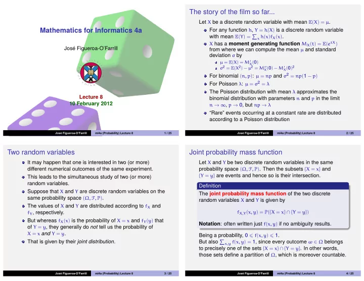
The story of the film so far... Let X be a discrete random variable with mean E ( X ) = µ . Mathematics for Informatics 4a For any function h , Y = h ( X ) is a discrete random variable with mean E ( Y ) = � x h ( x ) f X ( x ) . X has a moment generating function M X ( t ) = E ( e tX ) Jos´ e Figueroa-O’Farrill from where we can compute the mean µ and standard deviation σ by µ = E ( X ) = M ′ X ( 0 ) σ 2 = E ( X 2 ) − µ 2 = M ′′ X ( 0 ) 2 X ( 0 ) − M ′ For binomial ( n , p ) : µ = np and σ 2 = np ( 1 − p ) For Poisson λ : µ = σ 2 = λ The Poisson distribution with mean λ approximates the Lecture 8 binomial distribution with parameters n and p in the limit 10 February 2012 n → ∞ , p → 0, but np → λ “Rare” events occurring at a constant rate are distributed according to a Poisson distribution Jos´ e Figueroa-O’Farrill mi4a (Probability) Lecture 8 1 / 25 Jos´ e Figueroa-O’Farrill mi4a (Probability) Lecture 8 2 / 25 Two random variables Joint probability mass function It may happen that one is interested in two (or more) Let X and Y be two discrete random variables in the same different numerical outcomes of the same experiment. probability space ( Ω , F , P ) . Then the subsets { X = x } and { Y = y } are events and hence so is their intersection. This leads to the simultaneous study of two (or more) random variables. Definition Suppose that X and Y are discrete random variables on the The joint probability mass function of the two discrete same probability space ( Ω , F , P ) . random variables X and Y is given by The values of X and Y are distributed according to f X and f X , Y ( x , y ) = P ( { X = x } ∩ { Y = y } ) f Y , respectively. But whereas f X ( x ) is the probability of X = x and f Y ( y ) that Notation : often written just f ( x , y ) if no ambiguity results. of Y = y , they generally do not tell us the probability of X = x and Y = y . Being a probability, 0 � f ( x , y ) � 1. But also � That is given by their joint distribution . x , y f ( x , y ) = 1, since every outcome ω ∈ Ω belongs to precisely one of the sets { X = x } ∩ { Y = y } . In other words, those sets define a partition of Ω , which is moreover countable. Jos´ e Figueroa-O’Farrill mi4a (Probability) Lecture 8 3 / 25 Jos´ e Figueroa-O’Farrill mi4a (Probability) Lecture 8 4 / 25

Marginals Examples (Fair dice: scores, max and min) The joint probability mass function f ( x , y ) of two discrete We roll two fair dice. random variables X and Y contains the information of the Let X and Y denote their scores. The joint probability mass 1 probability mass functions of the individual discrete random function is given by variables. These are called the marginals : � 1 � � 36 , 1 � x , y � 6 f X ( x ) = f ( x , y ) and f Y ( y ) = f ( x , y ) . f X , Y ( x , y ) = 0, otherwise y x This holds because the sets { Y = y } , where y runs through all Let U and V denote the minimum and maximum of the two the possible values of Y , are a countable partition of Ω . 2 Therefore, scores, respectively. The joint probability mass function is � { X = x } ∩ { Y = y } . given by { X = x } =  1 y 36 , 1 � u = v � 6    and computing P of both sides: 1 f U , V ( u , v ) = 18 , 1 � u < v � 6  � �   0, otherwise f X , Y ( x , y ) . f X ( x ) = P ( { X = x } ) = P ( { X = x } ∩ { Y = y } ) = y y A similar story holds for { Y = y } . Jos´ e Figueroa-O’Farrill mi4a (Probability) Lecture 8 5 / 25 Jos´ e Figueroa-O’Farrill mi4a (Probability) Lecture 8 6 / 25 More than two random variables Examples Toss a fair coin. Let X be the number of heads and Y the 1 There is no reason to stop at two discrete random variables: we number of tails: can consider a finite number X 1 , . . . , X n of discrete random variables on the same probability space. They have a joint f X ( 0 ) = f X ( 1 ) = f Y ( 0 ) = f Y ( 1 ) = 1 probability mass function f X 1 ,..., X n : R n → [ 0, 1 ] , defined by 2 f X , Y ( 1, 0 ) = f X , Y ( 0, 1 ) = 1 f X , Y ( 0, 0 ) = f X , Y ( 1, 1 ) = 0 2 f X 1 ,..., X n ( x 1 , . . . , x n ) = P ( { X 1 = x 1 } ∩ · · · ∩ { X n = x n } ) and obeying Toss two fair coins. Let X be the number of heads shown 2 by the first coin and Y the number of heads shown by the � f X 1 ,..., X n ( x 1 , . . . , x n ) = 1 . second: x 1 ,..., x n f X ( 0 ) = f X ( 1 ) = f Y ( 0 ) = f Y ( 1 ) = 1 2 It has a number of marginals by summing over the possible f X , Y ( 0, 0 ) = f X , Y ( 1, 1 ) = f X , Y ( 1, 0 ) = f X , Y ( 0, 1 ) = 1 4 values of any k of the X i . Moral : the marginals do not determine the joint distribution! Jos´ e Figueroa-O’Farrill mi4a (Probability) Lecture 8 7 / 25 Jos´ e Figueroa-O’Farrill mi4a (Probability) Lecture 8 8 / 25

Independence Example (Bernoulli trials with a random parameter) second of the above examples , we saw that f X , Y ( x , y ) = f X ( x ) f Y ( y ) . Consider a Bernoulli trial with probability p of success. Let X In the and Y denote the number of successes and failures. Clearly This is explained by the fact that for all x , y the events { X = x } and { Y = y } are independent: they are not generally independent because X + Y = 1: so f X , Y ( 1, 1 ) = 0, yet f X ( 1 ) f Y ( 1 ) = p ( 1 − p ) . f X , Y ( x , y ) = P ( { X = x } ∩ { Y = y } ) Now suppose that we repeat the Bernoulli trial a random (independent events) number N of times, where N has a Poisson probability mass = P ( { X = x } ) P ( { Y = y } ) function with mean λ . I claim that X and Y are now independent! = f X ( x ) f Y ( y ) . We first determine the probability mass functions of X and Y . Conditioning on the value of N , Definition ∞ ∞ p x q n − x e − λ λ n � n � � � f X ( x ) = P ( X = x | N = n ) P ( N = n ) = Two discrete random variables X and Y are said to be n ! x n = x n = 1 independent if for all x , y , ∞ = ( λp ) x q m m ! λ m = ( λp ) x e − λ e λq = ( λp ) x � e − λ e − λp f X , Y ( x , y ) = f X ( x ) f Y ( y ) x ! x ! x ! m = 0 So X has a Poisson probability mass function with mean λp . Jos´ e Figueroa-O’Farrill mi4a (Probability) Lecture 8 9 / 25 Jos´ e Figueroa-O’Farrill mi4a (Probability) Lecture 8 10 / 25 Independent multiple random variables Example (Bernoulli trials with a random parameter – continued) One person’s success is another person’s failure, so Y also has Again there is no reason to stop at two discrete random a Poisson probability mass function but with mean λq . variables and we can consider a finite number X 1 , . . . , X n of Therefore discrete random variables. They are said to be independent when all the events { X i = x i } f X ( x ) f Y ( y ) = ( λp ) x e − λp ( λq ) y e − λq = e − λ λ x + y x ! y ! p x q y are independent. x ! y ! This is the same as saying that for any 2 � k � n variables X i 1 , . . . , X i k of the X 1 , . . . , X n , On the other hand, conditioning on N again, f X i 1 ,..., X ik ( x i 1 , . . . , x i k ) = f X i 1 ( x i 1 ) . . . f X ik ( x i k ) f X , Y ( x , y ) = P ( { X = x } ∩ { Y = y } ) for all x i 1 , . . . , x i k . = P ( { X = x } ∩ { Y = y }| N = x + y ) P ( N = x + y ) p x q y e − λ λ x + y � x + y � = ( x + y ) ! x = e − λ λ x + y x ! y ! p x q y = f X ( x ) f Y ( y ) Jos´ e Figueroa-O’Farrill mi4a (Probability) Lecture 8 11 / 25 Jos´ e Figueroa-O’Farrill mi4a (Probability) Lecture 8 12 / 25

Making new random variables out of old Proof Let X and Y be two discrete random variables and let h ( x , y ) be The cardinality of the set Z ( Ω ) of all possible values of Z is at any function of two variables. Then let Z = h ( X , Y ) be defined most that of X ( Ω ) × Y ( Ω ) , consisting of pairs ( x , y ) where x is a by Z ( ω ) = h ( X ( ω ) , Y ( ω )) for all outcomes ω . possible value of X and y is a possible value of Y . Since the Cartesian product of two countable sets is countable, Z ( Ω ) is Theorem countable. Z = h ( X , Y ) is a discrete random variable with probability mass Now, function � { Z = z } = { X = x } ∩ { Y = y } � f X , Y ( x , y ) f Z ( z ) = x , y h ( x , y )= z x , y h ( x , y )= z is a countable disjoint union. Therefore, and mean � � E ( Z ) = h ( x , y ) f X , Y ( x , y ) f Z ( z ) = f X , Y ( x , y ) . x , y x , y h ( x , y )= z The proof is mutatis mutandis the same as in the one-variable case. Let’s skip it! Jos´ e Figueroa-O’Farrill mi4a (Probability) Lecture 8 13 / 25 Jos´ e Figueroa-O’Farrill mi4a (Probability) Lecture 8 14 / 25 Functions of more than two random variables Proof – continued The expectation value is Again we can consider functions h ( X 1 , . . . , X n ) of more than two discrete random variables. � f Z ( z ) = zf Z ( z ) This is again a discrete random variable and its expectation is z given by the usual formula � � f X , Y ( x , y ) = z � E ( h ( X 1 , . . . , X n )) = h ( x 1 , . . . , x n ) f X 1 ,..., X n ( x 1 , . . . , x n ) x , y z h ( x , y )= z x 1 ,..., x n � h ( x , y ) f X , Y ( x , y ) = x , y The proof is basically the same as the one for two variables and shall be left as an exercise. Jos´ e Figueroa-O’Farrill mi4a (Probability) Lecture 8 15 / 25 Jos´ e Figueroa-O’Farrill mi4a (Probability) Lecture 8 16 / 25