The story of the film so far... We are developing a language to - PowerPoint PPT Presentation

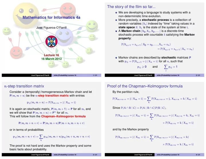
The story of the film so far... We are developing a language to study systems with a non-deterministic time evolution. Mathematics for Informatics 4a More precisely, a stochastic process is a collection of random variables { X t } indexed by “time” taking values in a state space S : X t is the state of the system at time t . José Figueroa-O’Farrill A Markov chain { X 0 , X 1 , X 2 , . . . } is a discrete-time stochastic process with countable S satisfying the Markov property : P ( X n + 1 = s n + 1 | X 0 = s 0 , . . . , X n = s n ) = P ( X n + 1 = s n + 1 | X n = s n ) Lecture 16 Markov chains are described by stochastic matrices P 16 March 2012 with p ij = P ( X n + 1 = j | X n = i ) for all n , such that � p ij � 0 and p ij = 1 j José Figueroa-O’Farrill mi4a (Probability) Lecture 16 1 / 21 José Figueroa-O’Farrill mi4a (Probability) Lecture 16 2 / 21 n -step transition matrix Proof of the Chapman–Kolmogorov formula Consider a (temporally) homogeneneous Markov chain and let By the partition rule, P ( m , m + n ) be the n -step transition matrix with entries � P ( X m + n + r = j , X m + n = k | X m = i ) P ( X m + n + r = j | X m = i ) = p ij ( m , m + n ) = P ( X m + n = j | X m = i ) k Since P ( A ∩ B | C ) = P ( A | B ∩ C ) P ( B | C ) , It is again an stochastic matrix, P ( m , m + 1 ) = P for all m , and we will show that P ( m , m + n ) = P n for all m . � P ( X m + n + r = j | X m = i ) = P ( X m + n + r = j | X m + n = k , X m = i ) This will follow from the Chapman–Kolmogorov formula k × P ( X m + n = k | X m = i ) P ( m , m + n + r ) = P ( m , m + n ) P ( m + n , m + n + r ) and by the Markov property or in terms of probabilities � � p ij ( m , m + n + r ) = p ik ( m , m + n ) p kj ( m + n , m + n + r ) P ( X m + n + r = j | X m = i ) = P ( X m + n + r = j | X m + n = k ) k k × P ( X m + n = k | X m = i ) The proof is not hard and uses the Markov property and some basic facts about probability. José Figueroa-O’Farrill mi4a (Probability) Lecture 16 3 / 21 José Figueroa-O’Farrill mi4a (Probability) Lecture 16 4 / 21

This allows us to express the probabilities at time n in terms of Corollary (of Chapman–Kolmogorov formula) the initial probabilities. Let π n ( i ) = P ( X n = i ) and consider the For all m , P ( m , m + n ) = P n . probability vector π n whose i th entry is π n ( i ) . Theorem Proof. For every n , m � 0 , π n + m = π m P n . By induction on n . For n = 1, we have that P ( m , m + 1 ) = P for all m (temporal homogeneity). Now for the induction step, Proof. suppose that P ( m , m + k ) = P k for all m and for all k < n . Then By the partition rule, by the Chapman–Kolmogorov formula for ( m , n − 1, 1 ) , � P ( X m + n = j ) = P ( X m + n = j | X m = i ) P ( X m = i ) P ( m , m + n ) = P ( m , m + n − 1 ) P ( m + n − 1, m + n ) i � p ij ( m , m + n ) π m ( i ) but P ( m , m + n − 1 ) = P n − 1 by the induction hypothesis, and = i P ( m + n − 1, m + n ) = P , whence P ( m , m + n ) = P n . which in terms of matrices is the product Notation π n + m = π m P ( m , m + n ) = π m P n We will let p ij ( n ) denote the matrix entries of P n . José Figueroa-O’Farrill mi4a (Probability) Lecture 16 5 / 21 José Figueroa-O’Farrill mi4a (Probability) Lecture 16 6 / 21 So in particular, π n = π 0 P n , so that the probabilities π n at time Example (Continued) n are the initial probabilities π 0 multiplied with the n th power of We proved earlier that the transition matrix. The transition matrices carry most of the information in the Markov chain. � � q q π n ( 0 ) = ( 1 − p − q ) n π 0 ( 0 ) − + p + q p + q Example � � p p Consider the general 2-state Markov chain π n ( 1 ) = ( 1 − p − q ) n π 0 ( 1 ) − + p + q p + q q and we can use this to calculate the n -step transition matrix P n . 1 − p 0 1 1 − q Notice that for any 2 × 2 matrix A : p � a 00 � � a 00 � a 01 a 01 ( 1, 0 ) = ( a 00 , a 01 ) ( 0, 1 ) = ( a 10 , a 11 ) a 10 a 11 a 10 a 11 with transition matrix whence setting π 0 ( 0 ) = 1 and π 0 ( 0 ) = 0 in turn we read off � p 00 � � 1 − p � p 01 p P = = � p 1 − q p 10 p 11 q + ( 1 − p − q ) n 1 � q � � p − p P n = − q p + q q p p + q q José Figueroa-O’Farrill mi4a (Probability) Lecture 16 7 / 21 José Figueroa-O’Farrill mi4a (Probability) Lecture 16 8 / 21

Stationary probability distributions Definition In the previous example, notice that if 2 > p + q > 0, then Let P be the transition matrix of a finite-state Markov chain. A | 1 − p − q | < 1 and hence ( 1 − p − q ) n → 0 as n → ∞ . Therefore probability vector π is a steady state distribution if πP = π . as n → ∞ , 1 � q � p P n → P ∞ = Questions p + q q p Do all (finite-state) Markov chains have steady state 1 This matrix P ∞ has the property that for any choice of initial distributions? probabilities π 0 = ( π 0 ( 0 ) , π 0 ( 1 )) , If so, is there a unique steady state distribution? 2 � � If so, will any initial distribution converge to the steady state q p 3 π 0 P ∞ = p + q , distribution? p + q � � q p The probability vector π = p + q , is stationary : π = πP . Answers p + q Indeed, Yes ! (but we will not prove it in this course) 1 Not necessarily. 2 � � � 1 − p � � � q p p q p p + q , p + q , = Not necessarily. 1 − q 3 p + q q p + q José Figueroa-O’Farrill mi4a (Probability) Lecture 16 9 / 21 José Figueroa-O’Farrill mi4a (Probability) Lecture 16 10 / 21 Uniqueness of steady state distribution Example Consider the following 2-state Markov chain Theorem � 1 0 � An irreducible finite-state Markov chain has a unique steady P = 0 1 0 1 1 1 state distribution. Then clearly every π obeys π = πP . Warning If the Markov chain has an infinite (but still countable) number Post-mortem of states, then this is not true; although there are theorems The problem here is that the Markov chain decomposes: not guaranteeing the uniqueness of a steady state distribution in every state is “accessible” from every other state. those cases as well. Definition This still leaves the question of whether in a Markov chain with a unique steady state distribution, any initial distribution A state j is accessible from a state i , if for some n � 0, eventually tends to it. p ij ( n ) > 0. A Markov chain is irreducible if any state is accessible from any other state; i.e., given any two states i , j , there is some n � 0 with p ij ( n ) > 0. José Figueroa-O’Farrill mi4a (Probability) Lecture 16 11 / 21 José Figueroa-O’Farrill mi4a (Probability) Lecture 16 12 / 21

Periods Example Consider the following 2-state Markov chain Definition A state i is said to be periodic with period k if any return visit to 1 � 0 1 � i occurs in multiples of k time steps. More precisely, let P = 1 0 0 1 k i = gcd { n | P ( X n = i | X 0 = i ) > 0 } 1 � � Then if k i > 1, the state i is periodic with period k i and if k i = 1, 1 2 , 1 Then there is a unique steady state distribution π = , but 2 the state i is aperiodic . A Markov chain is said to be aperiodic no other distribution converges to it. if all states are aperiodic. Post-mortem Theorem The problem here is that P 2 is the identity matrix, so every An irreducible, aperiodic, finite-state Markov chain has a unique distribution (except the steady state distribution) has “period” 2. steady state distribution π to which any initial distribution will eventually converge: for all π 0 , π 0 P n → π as n → ∞ . José Figueroa-O’Farrill mi4a (Probability) Lecture 16 13 / 21 José Figueroa-O’Farrill mi4a (Probability) Lecture 16 14 / 21 Example Example (Continued) Consider the following 3-state Markov chain The reason is the limit n → ∞ of P n exists: 2 8 3   13 13 13 1 P n →  2 8 3  2   13 13 13   2 8 3 1 1 1   13 13 13 0 2 4 4 1 4  1 3 1  P = And hence for any ( α , β , γ ) with α + β + γ = 1, 1   8 4 8 4   1 1 0 1 2 8 3   2 2 8 13 13 13 1 8 3 1  2 8 3  = ( α + β + γ )( 2  13 , 8 13 , 3 13 ) = ( 2 13 , 8 13 , 3 1 2 ( α , β , γ ) 13 )   4 2 13 13 13  2 8 3 13 13 13 1 2 It is actually enough to show that for some n � 1, P n has no Solving the equation πP = π for π = ( π 0 , π 1 , π 2 ) with � � zero entries! 13 , 8 2 13 , 3 π 0 + π 1 + π 2 = 1, we find π = . Moreover, any initial 13 distribution converges to it. José Figueroa-O’Farrill mi4a (Probability) Lecture 16 15 / 21 José Figueroa-O’Farrill mi4a (Probability) Lecture 16 16 / 21