the story of the film so far
play

The story of the film so far... We are discussing continuous-time - PowerPoint PPT Presentation

The story of the film so far... We are discussing continuous-time Markov processes known as birth and death processes , with state space Mathematics for Informatics 4a N = { 0, 1, 2, . . . } and two kinds of transitions: birth : n n + 1 with


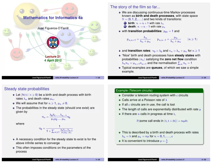
  1. The story of the film so far... We are discussing continuous-time Markov processes known as birth and death processes , with state space Mathematics for Informatics 4a N = { 0, 1, 2, . . . } and two kinds of transitions: birth : n → n + 1 with rate λ n 1 death : n → n − 1 with rate µ n 2 José Figueroa-O’Farrill with transition probabilities : p 01 = 1 and λ n µ n p n , n + 1 = p n , n − 1 = ( n � 1 ) λ n + µ n λ n + µ n and transition rates : ν 0 = λ 0 and ν n = λ n + µ n for n � 1 “Nice” birth and death processes have steady states with Lecture 21 probabilities ( π n ) satisfying the zero net flow condition 4 April 2012 λ n π n = µ n + 1 π n + 1 and the normalisation � n π n = 1 Typical examples are queues , of which we saw a simple example. José Figueroa-O’Farrill mi4a (Probability) Lecture 21 1 / 20 José Figueroa-O’Farrill mi4a (Probability) Lecture 21 2 / 20 Steady state probabilities Example (Telecom circuits) Let { N ( t ) | t � 0 } be a birth and death process with birth Consider a telecom routing system with c circuits rates λ n and death rates µ n . Calls arrive at a Poisson rate of λ We will assume that for n � 1, µ n � = 0. If all c circuits are in use, the call is lost The probabilities in the steady state (should one exist) are The length of calls are exponentially distributed with rate µ given by If there are n calls in progress at time t , π n = λ 0 λ 1 . . . λ n − 1 π 0 µ 1 µ 2 . . . µ n P ( some call ends in ( t , t + δt ]) = nµδt where 1 π 0 = 1 + � λ 0 λ 1 ... λ n − 1 n � 1 This is described by a birth and death process with rates µ 1 µ 2 ... µ n λ n = λ and µ n = nµ for n = 0, 1, . . . , c A necessary condition for the steady state to exist is for the It is convenient to introduce ρ = λ µ above infinite series to converge This often imposes conditions on the parameters of the process José Figueroa-O’Farrill mi4a (Probability) Lecture 21 3 / 20 José Figueroa-O’Farrill mi4a (Probability) Lecture 21 4 / 20
  2. Example (Telecom circuits – continued) Example (Telecom circuits – continued) The steady state probabilities are A call is lost if and only if all n ! µ n π 0 = ρ n λ n circuits are busy π n = ( n = 1, 2, . . . , c ) n ! π 0 In the steady state that happens with probability and π 0 is determined by the normalisation condition ρ c π c = � � 1 + ρ + 1 2 ρ 2 + · · · + 1 c ! c ! ρ c = 1 + ρ + 1 2 ρ 2 + · · · + 1 π − 1 c ! ρ c 0 The expression on the RHS is called Erlang’s loss formula , so that for n = 0, 1, . . . , c denoted ρ n π n = ρ c � � 2 ρ 2 + · · · + 1 1 + ρ + 1 c ! ρ c n ! E ( c , ρ ) = � � 2 ρ 2 + · · · + 1 1 + ρ + 1 c ! c ! ρ c José Figueroa-O’Farrill mi4a (Probability) Lecture 21 5 / 20 José Figueroa-O’Farrill mi4a (Probability) Lecture 21 6 / 20 Example (Telecom circuits – continued) Example (Telecom circuits – continued) In the limit c → ∞ of an infinite number of circuits We can rewrite E ( N ) in terms of the Erlang loss formula E ( c , ρ ) ∞ 1 � n ! ρ n = e ρ = π − 1 ⇒ π 0 = e − ρ = 0 c ρ n � n = 0 E ( N ) = ( n − 1 ) ! π 0 n = 1 and hence π n = e − ρ ρ n n ! , a Poisson distribution with rate ρ ! c − 1 ρ ℓ + 1 � = ℓ ! π 0 In the c → ∞ limit, the mean number of calls in the system ℓ = 0 is � � � c ρ ℓ ℓ ! − ρ c � E ( N ) = nπ n = ρ ℓ = 0 c ! = ρ n � c ρ ℓ ℓ = 0 ℓ ! For finite c , = ρ ( 1 − E ( c , ρ )) c ρ n � � E ( N ) = nπ n = ( n − 1 ) ! π 0 i.e., E ( c , ρ ) is the expected fraction of traffic lost n n = 1 José Figueroa-O’Farrill mi4a (Probability) Lecture 21 7 / 20 José Figueroa-O’Farrill mi4a (Probability) Lecture 21 8 / 20

  3. Example (M/M/s queues) Example (M/M/s queues — continued) This is a system where, unlike in the previous example, If there is a steady state, its probabilities are calls are not rejected when all servers are busy, but they  λ n n ! µ n π 0 , n = 1, . . . , s are sent to a queue  π n = We model this as a birth and death process with λ n  s ! s n − s µ n π 0 , n > s parameters: s : the number of servers λ : the arrival rate of calls and π 0 is determined by the normalisation condition µ : the service rate s − 1 λ k ∞ λ n The birth and death rates are then � � π − 1 = k ! µ k + 0 s ! s n − s µ n � n = s k = 0 nµ , n � s and λ n = λ µ n = sµ , n > s The (geometric) series convergence if λ < sµ , which is just the condition that the total service rate of the system exceeds the rate at which calls are entering José Figueroa-O’Farrill mi4a (Probability) Lecture 21 9 / 20 José Figueroa-O’Farrill mi4a (Probability) Lecture 21 10 / 20 Example (M/M/s queues — continued) Example (A shoe-shine shop) λ It is convenient to introduce ρ = sµ A shoe-shine shop has two In terms of ρ , chairs: one (chair 1) where the s − 1 s − 1 shoes are cleaned and the other ∞ ρ k s k + s s � s k k ! − s s � � 1 � � ρ n = π − 1 ρ k = 1 − ρ + (chair 2) where they are polished. 0 k ! s ! s ! n = s k = 0 k = 0 When a customer arrives, he goes initially to chair 1 and after Finally, his shoes are cleaned to chair 2.  ρ n s n 1 � , n � s   1 − ρ + � s − 1 n ! � sk k ! − ss  1 k = 0 ρ k s ! The service times at the two chairs are independent π n = s s ρ n 1 1 1  � , exponential random variables with means µ 1 and µ 2 . n > s   s ! 1 − ρ + � s − 1 � sk k ! − ss 1 k = 0 ρ k s ! Suppose that customers arrive according to a Poisson process with rate λ and that a customer will only enter the Of course, infinitely long queues are an idealisation: in system if both chairs are empty. practice, one has a finite buffer in which to store the calls in How can we model this as a Markov chain? the queue, with calls being lost if the buffer is full José Figueroa-O’Farrill mi4a (Probability) Lecture 21 11 / 20 José Figueroa-O’Farrill mi4a (Probability) Lecture 21 12 / 20

  4. Example (A shoe-shine shop — continued) Example (A shoe-shine shop — continued) Because the customer will not enter the system unless Because we have a transition 2 → 0, this is not a birth and both chairs are empty, there are at any given time either 0 death process or 1 customers in the system. Nevertheless we can use the zero net flow condition in If there is 1 customer in the system, then we would need to order to derive the steady-state probabilities: know which chair he’s in. 0 µ 2 This means that there are three states in the system: λ λπ 0 = µ 2 π 2 (0) the system is empty µ 1 π 1 = λπ 0 (1) a customer in chair 1 2 1 µ 2 π 2 = µ 1 π 1 (2) a customer in chair 2 µ 1 The transition probabilities are p 01 = p 12 = p 20 = 1 We can solve for π 1,2 in terms of π 0 , The times T 0 , T 1 and T 2 that the system spends on each state before making the transition to the next state, are � � π 1 = λ π 2 = λ 1 + λ + λ exponentially distributed with rates λ 0 = λ , λ 1 = µ 1 and π 0 , = 1 π 0 ⇒ π 0 = µ 1 µ 2 µ 1 µ 2 λ 2 = µ 2 , respectively. José Figueroa-O’Farrill mi4a (Probability) Lecture 21 13 / 20 José Figueroa-O’Farrill mi4a (Probability) Lecture 21 14 / 20 Example (The sex life of the amoeba) Example (A shoe-shine shop — continued) Finally, µ 1 µ 2 π 0 = µ 1 µ 2 + λ ( µ 1 + µ 2 ) λµ 2 π 1 = µ 1 µ 2 + λ ( µ 1 + µ 2 ) λµ 1 π 2 = µ 1 µ 2 + λ ( µ 1 + µ 2 ) amoebas can be in one of two states: either A or B There are other Markov processes which are closely linked an amoeba in state A will change to state B at an to birth and death processes, for which many of the exponential rate α techniques we have seen also apply an amoeba in state B will divide into two new amoebas of An interesting example is in the evolution of populations of type A at an exponential rate β single-celled organisms we assume amoebas are independent José Figueroa-O’Farrill mi4a (Probability) Lecture 21 15 / 20 José Figueroa-O’Farrill mi4a (Probability) Lecture 21 16 / 20

Download Presentation
Download Policy: The content available on the website is offered to you 'AS IS' for your personal information and use only. It cannot be commercialized, licensed, or distributed on other websites without prior consent from the author. To download a presentation, simply click this link. If you encounter any difficulties during the download process, it's possible that the publisher has removed the file from their server.

Recommend


More recommend