The story of the film so far... With every experiment we associate a - PowerPoint PPT Presentation

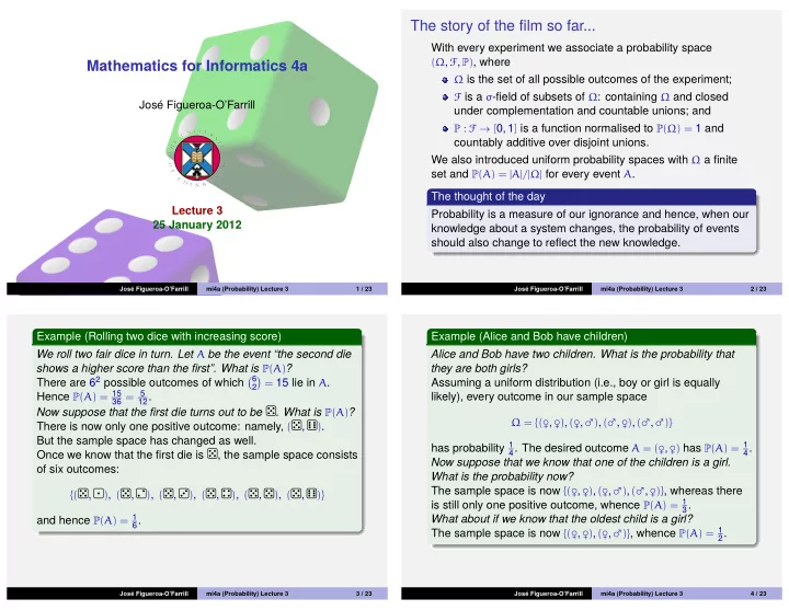
The story of the film so far... With every experiment we associate a probability space ( Ω , F , P ) , where Mathematics for Informatics 4a Ω is the set of all possible outcomes of the experiment; F is a σ -field of subsets of Ω : containing Ω and closed Jos´ e Figueroa-O’Farrill under complementation and countable unions; and P : F → [ 0, 1 ] is a function normalised to P ( Ω ) = 1 and countably additive over disjoint unions. We also introduced uniform probability spaces with Ω a finite set and P ( A ) = | A | / | Ω | for every event A . The thought of the day Lecture 3 Probability is a measure of our ignorance and hence, when our 25 January 2012 knowledge about a system changes, the probability of events should also change to reflect the new knowledge. Jos´ e Figueroa-O’Farrill mi4a (Probability) Lecture 3 1 / 23 Jos´ e Figueroa-O’Farrill mi4a (Probability) Lecture 3 2 / 23 Example (Rolling two dice with increasing score) Example (Alice and Bob have children) We roll two fair dice in turn. Let A be the event “the second die Alice and Bob have two children. What is the probability that shows a higher score than the first”. What is P ( A ) ? they are both girls? There are 6 2 possible outcomes of which � 6 � = 15 lie in A . Assuming a uniform distribution (i.e., boy or girl is equally 2 Hence P ( A ) = 15 36 = 5 12 . likely), every outcome in our sample space Now suppose that the first die turns out to be . What is P ( A ) ? Ω = { ( ♀ , ♀ ) , ( ♀ , ♂ ) , ( ♂ , ♀ ) , ( ♂ , ♂ ) } There is now only one positive outcome: namely, ( , ) . But the sample space has changed as well. has probability 1 4 . The desired outcome A = ( ♀ , ♀ ) has P ( A ) = 1 4 . Once we know that the first die is , the sample space consists Now suppose that we know that one of the children is a girl. of six outcomes: What is the probability now? The sample space is now { ( ♀ , ♀ ) , ( ♀ , ♂ ) , ( ♂ , ♀ ) } , whereas there { ( , ) , ( , ) , ( , ) , ( , ) , ( , ) , ( , ) } is still only one positive outcome, whence P ( A ) = 1 3 . and hence P ( A ) = 1 What about if we know that the oldest child is a girl? 6 . The sample space is now { ( ♀ , ♀ ) , ( ♀ , ♂ ) } , whence P ( A ) = 1 2 . Jos´ e Figueroa-O’Farrill mi4a (Probability) Lecture 3 3 / 23 Jos´ e Figueroa-O’Farrill mi4a (Probability) Lecture 3 4 / 23

Conditional probability Definition Let A , B be events. The conditional probability P ( A | B ) of the event of “ A occurs given that B occured” is P ( A | B ) = P ( A ∩ B ) P ( B ) assuming that P ( B ) > 0. This Dreyfus... Warning! P ( A | B ) � = P ( B | A ) , unless P ( A ) = P ( B ) . The incorrect equality formed the basis of the prosecution’s case in the infamous affaire Dreyfus in France at the turn of the 20th century. To find out more, visit my colleague Andrew Ranicki’s page on this ... not this Dreyfus! subject: http://www.maths.ed.ac.uk/~aar/dreyfus.htm . Jos´ e Figueroa-O’Farrill mi4a (Probability) Lecture 3 5 / 23 Jos´ e Figueroa-O’Farrill mi4a (Probability) Lecture 3 6 / 23 Conditional probability from uniform probability Conditional probability as relative frequency If ( Ω , F , P ) is a uniform probability space (e.g., Ω finite and all We repeat the experiment N times, with B occuring N ( B ) times. outcomes equally probable) and A , B are two events, we have Since we know that B occurs we are in one of those N ( B ) trials. The event A occurs in N ( A ∩ B ) of them, so the probability of A P ( A ) = | A | P ( B ) = | B | occuring given that B does is given by the limit N → ∞ of and | Ω | . | Ω | � N ( B ) N ( A ∩ B ) = N ( A ∩ B ) → P ( A ∩ B ) = P ( A | B ) . If B occurs, the possible outcomes are those in B and they N ( B ) P ( B ) N N remain equally likely with probability 1 / | B | . The event A occurs if and only if A ∩ B occurs, whence the probability that A occurs given that B occurs is � | B | | A ∩ B | = | A ∩ B | | Ω | = P ( A ∩ B ) = P ( A | B ) . | B | | Ω | P ( B ) We will now revisit the previous examples in the language of conditional probability. Jos´ e Figueroa-O’Farrill mi4a (Probability) Lecture 3 7 / 23 Jos´ e Figueroa-O’Farrill mi4a (Probability) Lecture 3 8 / 23

Example (Rolling two dice with increasing score) Example (Alice and Bob have children) Let A be the event “the second die shows a greater score than Let the first” and let B be the event “the first die shows a ”. A = { ( ♀ , ♀ ) } “both are girls” Then B = { ( ♀ , ♀ ) , ( ♀ , ♂ ) , ( ♂ , ♀ ) } “at least one is a girl” B = { ( , ) , ( , ) , ( , ) , ( , ) , ( , ) , ( , ) } C = { ( ♀ , ♀ ) , ( ♀ , ♂ ) } “the oldest is a girl” . A ∩ B = { ( , ) } Then P ( A | B ) = P ( A ∩ B ) = | A ∩ B | whence = 1 P ( A | B ) = P ( A ∩ B ) = | A ∩ B | 3 P ( B ) | B | = 1 6 . P ( B ) | B | and P ( A | C ) = P ( A ∩ C ) = | A ∩ C | = 1 2 P ( C ) | C | Jos´ e Figueroa-O’Farrill mi4a (Probability) Lecture 3 9 / 23 Jos´ e Figueroa-O’Farrill mi4a (Probability) Lecture 3 10 / 23 Conditional probability is a probability Example Let ( Ω , F , P ) be a probability space and let B ∈ F be an event A box contains a double-headed coin, a double-tailed coin and with P ( B ) > 0. Let P ′ ( A ) := P ( A | B ) . a conventional coin. A coin is picked at random, tossed and the Then P ′ is again a probability measure: result is a head. What is the probability that it is the P ′ : F → [ 0, 1 ] double-headed coin? Let D be the event that we did pick the double-headed coin and P ′ ( Ω ) = 1 let H be the event that the coin we picked and tossed, came up P ′ is countably additive over disjoint unions heads. We want to calculate P ( D | H ) . This means that all results proved for general probability There are 3 coins and hence 6 possible outcomes, of which 3 measures apply to the conditional probability as well. are heads. Therefore P ( H ) = 3 6 = 1 2 . In fact, we can define a new probability space ( B , F ′ , P ′ ) , where Of those 3 outcomes, two come from picking the double-headed coin, whence P ( D ∩ H ) = 2 6 = 1 3 . F ′ = { A ∩ B | A ∈ F} . Therefore P ( D | H ) = P ( D ∩ H ) � = 1 1 2 = 2 3 . 3 P ( H ) Recall that F ′ is again a σ -field (cf. Tutorial Sheet 1), only this time of subsets of B . Jos´ e Figueroa-O’Farrill mi4a (Probability) Lecture 3 11 / 23 Jos´ e Figueroa-O’Farrill mi4a (Probability) Lecture 3 12 / 23

Multiplication rule Extended multiplication rule definition of conditional probability there follows the From the Theorem Multiplication rule Let A 1 , A 2 , . . . , A n be events with P ( A 1 ∩ A 2 ∩ · · · ∩ A n ) > 0 . Then P ( A ∩ B ) = P ( A | B ) P ( B ) which holds even if P ( B ) = 0. P ( A 1 ∩ · · · ∩ A n ) = P ( A n | A n − 1 ∩ · · · ∩ A 1 ) × × P ( A n − 1 | A n − 2 ∩ · · · ∩ A 1 ) · · · P ( A 2 | A 1 ) P ( A 1 ) Example I have 5 red socks and 3 black socks in a drawer. I pick two socks at random. What is the probability that I get a black pair? Proof. Let P = “the pair is black” and B = “the first sock is black”. Then clearly P ⊂ B , so P = P ∩ B . Also P ( B ) = 3 8 and P ( P | B ) = 2 Just use that for k = 2, . . . , n , 7 , whence P ( A k ∩ · · · ∩ A 1 ) P ( A k | A k − 1 ∩ · · · ∩ A 1 ) = P ( A k − 1 ∩ · · · ∩ A 1 ) P ( P ) = P ( P ∩ B ) = P ( P | B ) P ( B ) = 2 7 × 3 8 = 3 28 . and multiply the terms in the RHS to obtain the LHS. Jos´ e Figueroa-O’Farrill mi4a (Probability) Lecture 3 13 / 23 Jos´ e Figueroa-O’Farrill mi4a (Probability) Lecture 3 14 / 23 Example Example A box contains 15 numbered balls: six balls have the number 1 , A bag contains 26 cards, each one with a letter in { a , b , c , . . . , z } . four balls the number 2 and five balls the number 3 . Suppose You take 7 cards at random without replacement. What is the we draw three balls without replacement. What is the probability probability that you can spell “dreyfus” with them? that we draw the balls in increasing numerical order? Let A i be the event that the i th card is one with a letter in Let A be event “first ball has number 1”, B the event “second { d , r , e , y , f , u , s } . We are after P ( A 1 ∩ A 2 ∩ · · · ∩ A 7 ) . We use the ball has number 2” and C the event “third ball has number 3”. extended multiplication rule: We want to compute P ( A ∩ B ∩ C ) . P ( A 1 ∩ · · · ∩ A 7 ) = P ( A 1 ) P ( A 2 | A 1 ) · · · P ( A 7 | A 6 ∩ · · · ∩ A 1 ) By the extended multiplication rule, = 7 26 × 6 25 × 5 24 × · · · × 1 20 P ( A ∩ B ∩ C ) = P ( C | A ∩ B ) P ( B | A ) P ( A ) 26 × 25 ×···× 20 × 19! 7 × 6 ×···× 1 = 19! where P ( A ) = 6 15 = 2 5 , P ( B | A ) = 4 14 = 2 7 and P ( C | A ∩ B ) = 5 13 , � − 1 � 26 1 657800 . = = whence 7 P ( A ∩ B ∩ C ) = 2 5 × 2 7 × 5 13 = 4 91 ≃ 4.4% Jos´ e Figueroa-O’Farrill mi4a (Probability) Lecture 3 15 / 23 Jos´ e Figueroa-O’Farrill mi4a (Probability) Lecture 3 16 / 23