
SLIDE 1
4/29/20 1
CSE-571 Robotics
SLAM: Simultaneous Localization and Mapping
Many slides courtesy of Ryan Eustice, Cyrill Stachniss, John Leonard
1
2
Given:
¤ The robot’s controls ¤ Observations of nearby features
Estimate:
¤ Map of features ¤ Path of the robot
The SLAM Problem
A robot is exploring an unknown, static environment.
2
3
SLAM Applications
Indoors Space Undersea Underground
3
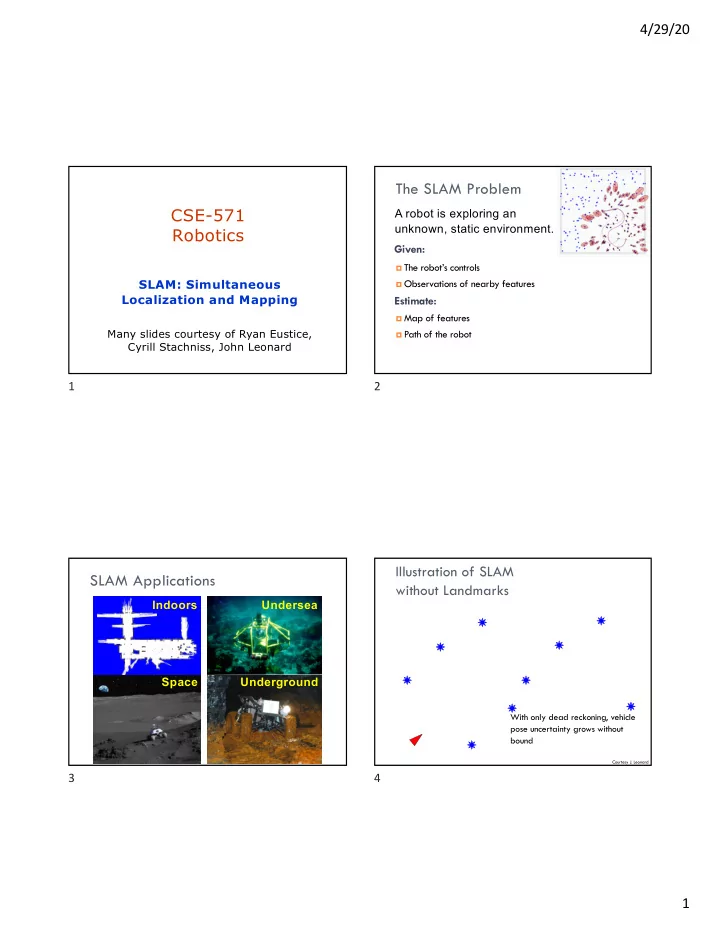
Illustration of SLAM without Landmarks
Courtesy J. Leonard