The Satisfiability problem Quest throughout history to establish an - - PowerPoint PPT Presentation

SLIDE 1

Heuristic Optimization

Lecture 8

Algorithm Engineering Group Hasso Plattner Institute, University of Potsdam

9 June 2015

Heuristic Optimization

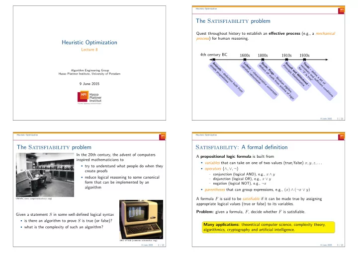
The Satisfiability problem

Quest throughout history to establish an effective process (e.g., a mechanical process) for human reasoning. 4th century BC

A r i s t

• t

l e – d e d u c t i

• n

b u i l t f r

• m

s i m p l e p r

• p
• s

i t i

• n

s

1600s

L e i b n i z – c h a r a c t e r i s t i c a u n i v e r s a l i s c a l c u l u s r a t i

• c

i n a t

• r

1800s

B

• l

e , F r e g e – B

• l

e a n a l g e b r a , d e d u c e a l l m a t h f r

• m

a x i

• m

s

• f

l

• g

i c

1910s

R u s s e l l a n d W h i t e h e a d – P r i n c i p i a M a t h e m a t i c a

1930s

T a r s k i – d e fi n e a s e t

• f

n e c e s s a r y a n d s u ffi c i e n t c

• n

d i t i

• n

s f

• r

“ F i s t r u e ”

9 June 2015 1 / 22 Heuristic Optimization

The Satisfiability problem

UNIVAC (www.computerhistory.org)

In the 20th century, the advent of computers inspired mathematicians to

• try to understand what people do when they

create proofs

• reduce logical reasoning to some canonical

form that can be implemented by an algorithm Given a statement S in some well-defined logical syntax

• is there an algorithm to prove S is true (or false)?
• what is the complexity of such an algorithm?

DEC VT100 (commons.wikimedia.org) 9 June 2015 2 / 22 Heuristic Optimization

Satisfiability: A formal definition

A propositional logic formula is built from

• variables that can take on one of two values (true/false) x, y, z, . . .
• operators {∧, ∨, ¬}

− conjunction (logical AND), e.g., x ∧ y − disjunction (logical OR), e.g., x ∨ y − negation (logical NOT), e.g., ¬x

• parentheses that can group expressions, e.g., (x) ∧ (¬x ∨ y)

A formula F is said to be satisfiable if it can be made true by assigning appropriate logical values (true or false) to its variables. Problem: given a formula, F, decide whether F is satisfiable. Many applications: theoretical computer science, complexity theory, algorithmics, cryptography and artificial intelligence.

9 June 2015 3 / 22

SLIDE 2

Heuristic Optimization

Satisfiability: Basics

A well-formed Boolean expression can be described by the grammar: expr ::= variable | expr ∧ expr | expr ∨ expr | (expr) | ¬expr The assignment of a Boolean variable v is a binding to a value in {0, 1}. If all variables in an expression are bound, the evaluation can be done recursively: E F E ∧ F E ∨ F (E) ¬E 1 1 1 1 1 1 1 1 1 1 1 1

9 June 2015 4 / 22 Heuristic Optimization

Definitions

The assignment of n Boolean variables can be represented as x ∈ {0, 1}n. Let F be a formula on n variables. We write F[x] ∈ {0, 1} as the evaluation of F under the assignment x ∈ {0, 1}n. Given a Boolean expression F on n Boolean variables, we say an assignment x ∈ {0, 1}n satsifies F if F[x] = 1. Example F = (¬x1 ∨ x2) ∧ ¬x1 ∧ (¬x3 ∨ ¬x1) x = (0, 0, 0), F[x] = ? x = (1, 0, 1), F[x] = ? 1

9 June 2015 5 / 22 Heuristic Optimization

Definitions

Two Boolean formulas E and F on n Boolean variables are said to be equivalent if ∀x ∈ {0, 1}n, F[x] = E[x]. In this case we write F ≡ E A literal: a variable v or its negation ¬v. A clause: a disjunction of literals, e.g., (x1 ∨ ¬x2 ∨ ¬x3 ∨ · · · ∨ xi) A formula F is said to be in conjunctive normal form (CNF) when F is written as a conjunction of clauses.

Lemma

For every well-formed formula F, there is a formula E such that (1) E is in CNF, and (2) F ≡ E. CNF form is much easier to work with!

9 June 2015 6 / 22 Heuristic Optimization

Is Satisfiability easy or hard?

Let F be the set of all admissible formulas. We consider some subsets of F: F1 formulas satisfied when all variables are set true (false). F2 formulas F ≡ E, where E is in CNF and each clause contains at most one positive (resp., negative) literal. F3 formulas F ≡ E, where E is in CNF and each clause contains ≤ 2 literals. F4 formulas F ≡ E, where E is conjunction of exclusive-or clauses. Horn formulas 2-CNF formulas Affine formulas

Schaefer’s Dichotomy Theorem (1978)

• 1. Every formula F ∈ (F1 ∪ F2 ∪ F3 ∪ F4) can be decided in time polynomial

in the length of F.

• 2. The class F \ (F1 ∪ F2 ∪ F3 ∪ F4) is NP-complete.a

aTechnical note: Schaefer’s approach is constrained to classes that can be

recognized in log space.

9 June 2015 7 / 22

SLIDE 3

Heuristic Optimization

Resolution for first-order logics

1958 Martin Davis & Hilary Putnam developed a resolution procedure for first-order logic (quantifiers allowed) Herbrand’s theorem: if a first-order formula is unsatisfiable then it has some ground formula in propositional logic (quantifier-free) that is unsatsifiable.

Davis-Putnam procedure

• 1. Generate all propositional ground instances
• 2. Check if each instance F is satisfiable

The main innovation is in (2), where we must solve Satisfiability Given a propositional logic formula F in CNF, assign variables using three reduction rules.

9 June 2015 8 / 22 Heuristic Optimization

Davis-Putnam procedure

Rule 1: unit rule (x1 ∨ ¬x2 ∨ x3) ∧ (x2 ∨ ¬x3) ∧ (x1) ∧ (¬x1 ∨ x4 ∨ x3) ∧ (¬x2) set x1 = 1 (x2 ∨ ¬x3) ∧ (x4 ∨ x3) ∧ (¬x2) set x2 = 0 Reduced formula: (¬x3) ∧ (x4 ∨ x3) For each unit clause (ℓ)

• set ℓ to 1, ¬ℓ to 0
• remove clauses containing ℓ, delete occurrences of ¬ℓ
• repeat until no unit clauses exist

9 June 2015 9 / 22 Heuristic Optimization

Davis-Putnam procedure

Rule 2: pure literal rule (x1 ∨ ¬x3 ∨ x4) ∧ (¬x3 ∨ ¬x2) ∧ (x1 ∨ x2) ∧ (¬x2 ∨ ¬x4) ∧ (x3 ∨ ¬x4) pure literal set x1 = 1 pure literal set x2 = 0 Reduced formula: (x3 ∨ ¬x4) For each pure literal ℓ

• set ℓ to 1, ¬ℓ to 0
• remove clauses containing ℓ
• repeat until no pure literals exist

9 June 2015 10 / 22 Heuristic Optimization

Davis-Putnam procedure

Rule 3: rule for eliminating atomic formulas (ground resolution) (x ∨ ℓ1,1 ∨ · · · ∨ ℓ1,k1) ∧ (¬x ∨ ℓ2,1 ∨ · · · ∨ ℓ2,k2) ∧ C When x = 0, (ℓ1,1 ∨ · · · ∨ ℓ1,k1) must be true When (x = 1, ℓ2,1 ∨ · · · ∨ ℓ2,k2) must be true (ℓ1,1 ∨ · · · ∨ ℓ1,k1 ∨ ℓ2,1 ∨ · · · ∨ ℓ2,k2) ∧ C Replace (x ∨ A) ∧ (¬x ∨ B) ∧ C with (A ∨ B) ∧ C as long as there are no ℓ1,i ∈ A, ℓ2,j ∈ B that are complementary

9 June 2015 11 / 22

SLIDE 4

Heuristic Optimization

Using memory wisely

In 1962, Loveland and Logemann tried to implement DP procedure on an IBM 704, but found that it used too much RAM.

IBM 704 at NASA in 1957 (commons.wikimedia.org)

Rule 3a: splitting rule From (x ∨ A) ∧ (¬x ∨ B) ∧ C, create a pair of separate formulasa (A ∧ C), (B ∧ C). Recursively check (A ∧ C) and (B ∧ C) for satisfiability.

awhere A, B and C don’t contain any occurrences of the variable x

L&L insight: keep a stack for formulas in external storage (tape drive) so the formulas in RAM don’t get too large.

9 June 2015 12 / 22 Heuristic Optimization

A closer look at the splitting rule:

(x ∨ A) ∧ (¬x ∨ B) ∧ C

split

= = ⇒ (A ∧ C), (B ∧ C) F

split

= = ⇒ F ′, F ′′ F

A formula containing at least one occurrence of a variable x set x ← 1 remove clauses containing x remove occurrences of literal ¬x

F ′ := F

• x=1

set x ← 0 remove clauses containing ¬x remove occurrences of literal x

F ′′ := F

• x=0

Observation:

• If F ′ or F ′′ contain an empty clause: then unsatisfied
• If F ′ or F ′′ contain no clauses: then satisfied

9 June 2015 13 / 22 Heuristic Optimization

Davis-Putnam-Logemann-Loveland (DPLL)

Davis-Putnam procedure with Logemann-Loveland enhancement (splitting rule)

DPLL(F)

Input: A set of clauses F Output: A truth value if F is a consistent set of literals then return true; if F contains an empty clause then return false ; for each unit clause (ℓ) in F do F ← unit-propagate(ℓ, F); end for each pure literal ℓ in F do F ← pure-literal-assign(ℓ, F); end ℓ ← choose-literal(F); return DPLL(F ∧ ℓ) ∨ DPLL(F ∧ ¬ℓ);

9 June 2015 14 / 22 Heuristic Optimization

DPLL search space

F F ′ . . . . . . . . . . . . F ′′ . . . . . . . . . . . . Total size of search tree?

n

• i=0

2i = 2n+1 − 1 How can we reduce the total number of nodes expanded?

9 June 2015 15 / 22

SLIDE 5

Heuristic Optimization

DPLL heuristics: Branching policies

Pick a good variable on which to branch Come up with a scoring function score(ℓ) that gives a value for picking a variable that makes ℓ true. Some scoring functions: max(ℓ) # occurrences of ℓ in F. Idea: Picking ℓ to maximize max(ℓ) satisfies as many clauses as possible. moms(ℓ) # occurrences of ℓ in F appearing in clauses of minimum size. Idea: reducing minimum clauses can lead to a unit-propagation sooner or reveal a contradiction faster mams(ℓ) := max(ℓ) + moms(¬ℓ). Idea: satisfy as many clauses as possible, create as many minimum-size clauses as possible

9 June 2015 16 / 22 Heuristic Optimization

DPLL heuristics: Branching policies

Jeroslow-Wang: jw(ℓ) :=

C∋ℓ 2−|C|.

Idea: exponential weighting: smaller clauses have more weight than larger ones. up(ℓ) # of unit propagations triggered by setting ℓ = true. adaptive learning: adapt branching rule during execution

9 June 2015 17 / 22 Heuristic Optimization

DPLL heuristics: Clause learning

When unit propagation results in a conflict (produces an empty clause),

• analyze the unit propagation process that resulted in the conflict
• add a new clause to the formula that explains and prevents repeating the

same conflict later in the search (x1 ∨ ¬x4 ∨ ¬x6) ∧ (¬x5 ∨ x6) ∧ (¬x5 ∨ x2 ∨ x4) ∧ (x3 ∨ x5) branches taken so far: set x1 = 0 set x2 = 0 set x3 = 0 (¬x4 ∨ ¬x6) ∧ (¬x5 ∨ x6) ∧ (¬x5 ∨ x4) ∧ (x5)

Unit propagation

(¬x4 ∨ ¬x6) ∧ (x6) ∧ (x4) (¬x6) ∧ (x6)

Contradiction!

9 June 2015 18 / 22 Heuristic Optimization

DPLL heuristics: Clause learning

branches taken so far: set x1 = 0 set x2 = 0 set x3 = 0 We can conclude the branch x1 = 0, x2 = 0, x3 = 0 leads to an unsatisfied formula In other words, (x1 = 0) ∧ (x2 = 0) ∧ (x3 = 0) = ⇒ (F = 0) ≡(F = 1) = ⇒ ¬ ((x1 = 0) ∧ (x2 = 0) ∧ (x3 = 0)) (contrapositive) ≡(F = 1) = ⇒ (x1 = 1) ∨ (x2 = 1) ∨ (x3 = 1) So in order for F to be satisfied, (x1 ∨ x2 ∨ x3) must be true. Learned clause: F ′ := F ∧ (x1 ∨ x2 ∨ x3) Note: many very sophisticated procedures for analyzing the structures of contradictions exist.

9 June 2015 19 / 22

SLIDE 6

Heuristic Optimization

A local search algorithm

DPLL: construct an assignment from scratch Another approach: start from a complete assignment. While not satisfied, make some small change. Repeat.

Random local search algorithm for Satisfiability

Choose x ∈ {0, 1}n uniformly at random; while F is not satisfied do y ← x; Choose C ∈ F not satisfied by x; Choose a literal ℓ ∈ C uniformly at random; Let i be the index such that {xi, ¬xi} ∋ ℓ; y[i] ← 1 − y[i]; end

9 June 2015 20 / 22 Heuristic Optimization

How efficient is the random local search algorithm?

• Theorem. (Papadimitriou, 1991)

Let F ∈ F3 (formulas that have at most two literals per clause). If F is satisfiable, then the local search algorithm finds the satisfying assignment in O(n2) time in expectation. Proof sketch. Gambler’s ruin Ne 0 e 1/2 +1e 1/2 −1e Expected flips until win/loss: O(N 2)

• Let x⋆ := satisfying assignment, x := be the current assignment.
• For any clause C ∈ F not satisfied by x, at least one of the values x[i]

doesn’t match the value in x⋆[i].

• Probability to pick that variable ≥ 1/2.
• Move closer to x⋆ with probability ≥ 1/2 (further away w/ prob. ≤ 1/2).

9 June 2015 21 / 22 Heuristic Optimization

k-CNF formulas

What about k-CNF formulas for k > 2? Run local search algorithm, starting from a new random solution every O(n) steps.

• Theorem. (Sch¨
• ning, 1991)

Let F be a k-CNF formula. If F is satisfiable, then the (restarting) local search algorithm finds the satisfying assignment in T steps where T is within a polynomial factor of (2(1 − 1/k))n. For 3-CNF formulas: (1.333)n Current best-known bound1 for 3-SAT: O(1.308n)

1Timon Hertli, FOCS 2011

9 June 2015 22 / 22