The relational data model and relational algebra 1 Preliminaries The - - PDF document

The relational data model and relational algebra

1 Preliminaries

The early days of database engines (1960’s) saw several competing “data models” (the formal specifications for how the system represents and reasons about data). Academic researchers had proposed several models that were rich, expressive, and provided admirable data independence, but that were impossible to implement efficiently. The models used by working systems, on the other hand, tended to be very limited. The “hierarchical” and “network” models were two of the most popular. Both

• ffered excellent runtime performance—when used properly—but left nearly everything up to the

application developers unlucky enough to work with them. In particular, these simple models provided very little data independence, so any change to the way data was stored required corresponding changes to the applications using that data.

1.a Hierarchical model

The hierarchical model assumes a database schema where all relationships between different objects can be represented as a tree. This assumption was often true for early database workloads such as flight reservations, banking and commerce: Customers make orders that contain items, airlines sell seats on flights to customers, and banks have branches that serve customers who hold accounts. For example, suppose we want to create an application that tracks student jobs on or near campus, with the following data:

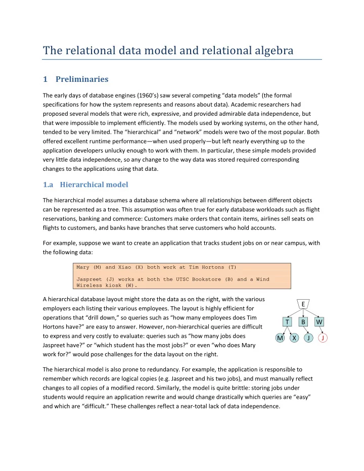
Mary (M) and Xiao (X) both work at Tim Hortons (T) Jaspreet (J) works at both the UTSC Bookstore (B) and a Wind Wireless kiosk (W).

A hierarchical database layout might store the data as on the right, with the various employers each listing their various employees. The layout is highly efficient for

• perations that “drill down,” so queries such as “how many employees does Tim

Hortons have?” are easy to answer. However, non‐hierarchical queries are difficult to express and very costly to evaluate: queries such as “how many jobs does Jaspreet have?” or “which student has the most jobs?” or even “who does Mary work for?” would pose challenges for the data layout on the right. The hierarchical model is also prone to redundancy. For example, the application is responsible to remember which records are logical copies (e.g. Jaspreet and his two jobs), and must manually reflect changes to all copies of a modified record. Similarly, the model is quite brittle: storing jobs under students would require an application rewrite and would change drastically which queries are “easy” and which are “difficult.” These challenges reflect a near‐total lack of data independence.

M X T J B J W E

1.b Network model

The network model generalizes the hierarchical model to represent relationships as directed graphs rather than trees. Doing so improves efficiency significantly: an application can easily add connections between records in order to accelerate important queries. For example, a possible network model version of our employee database might look like the one shown to the right. Questions about employers are still easy to express and evaluate, and now queries about employees also become efficient. The model also removes the need to store so many redundant copies of records. Although an improvement on the hierarchical model, the network model still provides inadequate data

• independence. The application remains responsible to define and maintain links between records, and

the system provides no way to verify systematic problems like missing (or extra) links; these are difficult to prevent or detect (e.g. we added a new employer to the database but forgot to add them to the list of employers, or linking a student to their employer, but forgetting the reverse link connecting employer to student). As the number of links grows, bugs frequently arise in applications that modify records from several points in the code. Further, changes to the linking strategy still require application changes, making it very costly to experiment with the data layout.

1.c Relational model

In the early 1970’s Edgar Codd proposed the relational model, which took a very different approach to data models. Unlike the competition of the day, it provided two key innovations:

• 1. A declarative framework applications use to specify the objects to be stored, the relationships

between various types of objects, and all accesses to those objects.

• 2. A formal system for specifying data (and operations on that data) that allows both the user and

database engine to reason about correctness, and to manipulate queries mechanically. The first point is important because it provides data independence: Minor changes, such as changing the type of a field or adding/removing/renaming fields from the database, require only focused changes to the application (e.g. to use the new name, stop using the deleted field, etc.). Changes to the underlying data representation are completely hidden from the application, other than their impact on

• performance. Further, because the database engine is explicitly aware of relationships between objects,

it can ensure those relationships are stored and updated properly, while relieving the application from most of the associated housekeeping.

B W J M X T E S

The second point is crucial because it gives the database engine a means to apply aggressive

• ptimizations to the (declaratively‐specified) operations requested by applications, while proving that

the end result is the same. These optimizations can include mechanically rewriting the query to access the underlying data more efficiently, select algorithms that perform less work (often by several orders of magnitude), and taking into account available resources such as available memory and parallelism.1 The next section introduces this formal model, which is known as relational algebra. Conceptually, the relational model is quite simple. It consists of “relations” (tables) of tuples (objects), each containing one or more fields (atomic values). Error! Reference source not found. gives an

• verview of the relational model, along with some important terminology. The relational model is set‐

based: the schema is a set of attributes (each naming a particular column), and the body of a relation is a set of tuples.2 This basis in sets is the primary source of data independence: Attributes within a tuple are accessed by name, and each tuple within a relation is unique. Meanwhile, the database engine is free to store tuples and their attributes in any order, and need not even store them together at all… as long as it can re‐assemble them when needed.

WARNING: Sets do not define any concept of “order” among their

• elements. As a notational aid, we might refer to some tuple as

“row ten” or attribute “x” as the third column, but it must be understood that those numberings are for convenience only (not part of the formal model) and the number assigned to a given tuple or attribute is subject to change without notice in any real system. In other words, row “ten” of a relation is simply whichever tuple the database engine happens to return after it has already delivered nine others, and it could legally return those tuples in a different order next time you ask for them.

1 Database languages were among the first and biggest successes in automatic parallelization, for example. 2 Tuples are not sets of values, however; they’re more like unordered lists.

Figure 1. Overview of the relational model

R a1 … ... ... am t1 v1,1 … … tn vn,m Tuple (row) Attribute Body Schema (heading) Relation name Value (field, atom) Cardinality: n=|R| Arity: m=|schema(R)| Sub‐tuples not allowed Set of attributes Set of tuples Column Position number (notational aid only)

Because the relational model is amenable to aggressive optimization while still providing data independence, vendors were able to produce efficient implementations whose good performance and ease of use quickly eclipsed other data models for all but the most specialized settings; today it remains by far the most popular means to store and manipulate structured data.3

2 Relational algebra

The core of the relational data model is a formal algebra for manipulating data in that model. Not surprisingly, it’s called “relational algebra,” and operations take finite relations as input and produce finite relations as output, rather than working with individual tuples. This section will define the algebra and briefly outline its primitive operations.

2.a Integer arithmetic: a familiar algebra

Formally, an algebra is a set of operations over a closed domain of values, together with a set of laws that define how those operations can be combined and manipulated. To illustrate this concept in more familiar terms, we will briefly examine the algebra of integer arithmetic. The domain of integer arithmetic is the integers (both positive and negative), with two of those values (‘0’ and ‘1’) having special significance. The algebra defines three primitive operations: addition (binary ‘+’), multiplication (binary ‘*’), and negation (unary ‘‐’).4 Addition and multiplication are both associative and commutative, and have the property that x+0 = x = 0+x and x*1 = x = 1*x for all x; negation has the property that x + ‐x = 0 for all x. Multiplication also distributes across addition: (x+y)*z = x*z + y*z. Operators can be combined into expressions, with evaluation order defined by parentheses: w+(x+(y+z)) evaluates from right‐to left, while ((w+x)+y)+z; laws of precedence specify the evaluation order when parentheses do not impose one: ‐x*y+z is equivalent to ((‐x)*y)+z. Expressions can be depicted as trees, with values as leaves, operators as internal nodes, and the final result appearing at the root. The graphical representation is often far easier to read than the fully parenthesized version; compare the example above‐right to (e+((2*a)+((c‐d)*5))), for example.

2.b Defining relational algebra

Like arithmetic, relational algebra consists of a closed domain and a few core operations.

3 We will only briefly touch on unstructured and semi‐structured data (such as text) in this course 4 Note that division is not part of the arithmetic of integers… why is that? Hint: what does 5/2 equal?

2 e ‐ a * c d * 5 + +

The domain is finite relations: sets of tuples having finite cardinality and arity. Attributes are usually typed, but need not be (the sqlite database engine uses untyped attributes, for example). Relational algebra consists of several primitive operations: selection (σ), projection (π), rename (ρ), set union (∪), set difference (‐), and Cartesian product (⨯). These operators can be combined to synthesize all other operations used in relational algebra.

3 Relational operators

3.a Selection (σ)

Selection returns the subset of tuples that satisfy a given predicate. It makes a convenient way to eliminate unwanted rows from a relation, and to isolate the tuples we are interested in. Selection does not change the schema of the relation it impacts.

3.b Projection (π)

Projection removes specific, unwanted attributes (columns) from a relation. The

• utput relation’s cardinality and arity can both shrink as a result of projection:

the output schema is a subset of the input relation (missing the attributes that were removed), and the number of tuples may decrease if the projection produced duplicates (recall that relations are sets, and sets do not contain duplicates).

3.c Rename (ρ)5

Rename is a very simple operator, whose only purpose is to change the name of

• ne or more attributes in a relation. Although this sounds trivial, it turns that many

common relational algebra operations are difficult to describe formally without it. For example, rename gives a clean way to make two relations union‐compatible, so long as the two schemata differ only in one or more attribute names.

3.d Union (∪) and difference (‐ or /)6

5 It could be argued that rename is not a primitive operation (it doesn’t do anything to the data), but its function is

important and cannot be emulated with the others.

6 Set intersection is not a primitive operation, because it can be synthesized from other operations (which ones?)

σ π ρ

Relations inherit all the familiar set operators, including union and difference. They work exactly the same way as a traditional set, with the additional restriction that their inputs must have matching schemata: two relations containing identical tuples but different attribute names are not the same, and would not be combined using set operations (though a rename operation might make them compatible). Union (depicted top‐right) returns a new relation containing every tuple that appears in either input relation, without duplicates in case the tuple appears in both. Difference (bottom‐right) returns a new relation containing every tuple from the left relation that does not appear in the right relation. No tuple from the second relation appears in the

• utput.

3.e Cartesian product (⨯)

The set operators are sometimes called “additive” because they have an effect on relation cardinality that resembles addition or subtraction : union “adds” tuples together and difference “subtracts” them. By this way of thinking, Cartesian product is like multiplication: it takes relations, with cardinality N and M, and returns a new relation with cardinality N*M. Unlike the additive operators, however, Cartesian product requires disjoint input schemas; the output schema is the union of its inputs, and each tuple is a concatenation of two inputs tuples. In fact, this is where the multiplication‐like behavior arises: the operator’s output contains the concatenation of every possible pairwise combination of tuples from the input relations. The figure on the right depicts this behavior

• graphically. Note that, by definition, the result is a set (no duplicates) because it contains every unique

combination of unique elements from two sets. Cartesian product is seldom used directly (it is extremely expensive to evaluate), but it provides a useful way to describe other, more useful, operators that we will discuss later.

4 Relational expression trees

Just as we can represent arithmetic using expression trees, it can be very useful to draw relational algebra expressions in tree form (linear and fully parenthesized forms tend to be used less because they can be hard to read). Consider the RA expression on the right: it takes four relations as input (A, B, R, S) which would correspond to numbers in arithmetic. It uses several different relational operators, some unary (e.g. σ) and several binary (e.g. ⨯). Note that there are no ternary operators in relational algebra: if you want to union three sets, you must union two of them and then union the result. Because the various operators constrain their input and output schemas, we can infer quite a bit about the input relations from the diagram: A’s schema must have at least some columns

U / 3 2 1 C B A x C B A C B A C B A 3 2 1 3 2 1 3 2 1

‐ A πx,y,z R S ⨯ B ∪ σx<3 and y > 2 ρx=m

besides x, y, and z (else we would not need to project them away); R and S cannot contain attribute x (because the other input to the Cartesian product contains attribute x), and B must contain attribute m (which is renamed to x before the relation becomes input to a Cartesian product); R and S have the same schema, but we cannot determine whether they contain attributes y, z or both; B could contain y

• r z, but not both, because R and S must contribute at least one attribute to the Cartesian product. The
• utput relation’s schema contains attributes x, y and z, and at least x and y have numeric types. The

selection even puts some restrictions on the values x and y can take in the output relation. Finally, we can see from the diagram that the tree admits some manipulation: it would be safe (and perhaps even desirable) to “push” the selection on x and y lower down in the plan: selection and union do not interfere with each other, nor do selection and Cross product. We would have to be careful about selecting away tuples before they participate in a difference, however. What about rename? Could we delay the rename of B’s m attribute until after the Cartesian product? The answer is “yes” because we know that neither R nor S contains an attribute m that might conflict, and we just need to ensure the rename occurs before the relation arrives as input to the union. Database query optimizers explore these kinds possibilities of rewriting (and many other tricks), in search of query plans that require less work than the one the user provided—orders of magnitude less work in some cases.

5 Relational algebra in practice

The theory of relational algebra is quite powerful, but it turns out to have several annoying limitations in practical applications. The limitations relate to both functionality and matters of presentation. This section will explore several of these practicalities and how we deal with them.

5.a “Extended” projection

As another practicality, it is often more interesting to see which columns a projection removes, rather than those it preserves (perhaps to save writing when there are many more of the latter than of the former). We can express this easily enough by placing a minus sign in front of column names to be

• eliminated. For example, given the relation R(w,x,y,z), the projection ,, could be written more

concisely as . Practical queries often require the use of an attribute whose value is computed from other values, rather than stored. Examples might be computing the total payment due, given a price and a tax rate (e.g. T = p*(1+t)), or the fuel efficiency of a vehicle when we know distance traveled and quantity of fuel

• consumed. We extend relational algebra to capture these computations with an “extended” version of

the projection operator; the previous examples would be rendered as ∗ and ∗. By default, we assume that extended projection does not remove any other attributes from the relation, reflecting its additive nature. The two notations can be usefully combined, e.g. ∗,, specifies a projection that computes attribute T while removing attributes p and t (from which T was computed). If we desire to remove all non‐computed attributes from an extended projection, we can adopt the star (*) notation

from SQL: ∗,∗ or simply follow the extended projection with a normal one that preserves

• nly the desired attributes.

5.b Sorting (τ)

Relational algebra, being set‐based, makes no promises about the order in which tuples are returned to the user. The user cannot even assume the same query, issued twice, would return the same ordering both times. In real life, we extend the algebra with a sorting operator, τ , parameterized by the columns

• n which to sort (in decreasing order of importance). For example, the relation shown on the left of

Figure 2 might be produced by ,; note that the last column is only nearly sorted. Sorting is quite useful in practice, even if it technically produces results outside the domain of relational algebra:7 Users often require sorted answers (names in alphabetical order, newer emails first, lowest price first, etc.). Further, several relational operators (including the set operators) can be implemented very efficiently if their inputs are known to be sorted appropriately. If the user explicitly requests sorting, the query optimizer can exploit that ordering to make other parts of the plan more efficient. Sometimes, the benefit of having sorted input available outweighs the cost of sorting the input, which may cause the query optimizer to insert “unnecessary” sort operations for performance reasons. For example, suppose we wished to compute the intersection of two lists: A=[1, 2, …, 99999, 1000000] and B=[500000, 500001, …, 1499999, 1500000]; if the lists were unsorted, we would require some large data structure to hold the elements from one side or the other, while testing against the other set of

• tuples. With sorted inputs, however, it suffices to stream through the two inputs, comparing the head of

each stream for matches and advancing the smaller of the two after each step.

5.c Duplicates

Perhaps the biggest restriction in relational algebra is that relations must be sets. Users often need duplicates to be preserved (because they are interested in how many times an event occurred, for example), and will view set semantics as a bug, not a feature. Further, even if the user does not care about duplicates, the obvious and efficient implementation of some relational operators—notably π and ∪—can produce duplicates because they treat relations as lists of tuples. For example, a straightforward projection algorithm would examine tuples one by one, removing unwanted columns. If some of the unwanted columns were part of the relation’s key (needed to uniquely identify each tuple), then the

• utput could contain duplicates, as can be seen in the figure below.

7 Although sorting a relation technically removes it from the domain of relational algebra, the distinction matters

very little in practice. The database engine can always “forget” a relation is sorted and treat it as a set again.

Figure 2. Projection can create duplicates if implemented naïvely

Even in the best case, where the relation is already sorted, a proper projection operator would have to record the previous tuple in order to detect and eliminate runs of identical tuples; in the common case where tuples are stored in arbitrary order (set semantics!), duplicate elimination requires even more

• work. Union suffers a similar problem: duplicate elimination is relatively easy as long as both input

relations are sorted, but requires significant extra work in the general case.

5.d Bag semantics and the distinct operator (δ)

To avoid these difficulties with duplicates, we extend relational algebra to use relations that are bags rather than sets. Like sets, bags (sometimes called “multisets”) are collections that impose no particular

• rdering on their elements, but unlike sets they allow duplicates. The introduction of bag semantics has

several minor impacts on the formal relational algebra:  A new distinct operator (δ) allows users to impose set semantics when desired  The efficient “projection” algorithm outlined in Figure 2 becomes correct  Union becomes list concatenation, also efficient  Union and intersection no longer distribute8  Difference and intersection behave differently for bags than for sets (but see discussion below) Of these, the distinct operator and union‐as‐concatenation are the most visible; the other changes are

• nly of interest to the database optimizer, which can use more efficient operations but loses the

distributive law. Note that modern database engines continue to use set versions of intersection, difference and union, though users can request bag union if they desire (using the so‐called “union all” operator). In contrast, projection allows duplicates unless the user explicitly passes the result through δ. This is partly due to the principle of least surprise. Users are not surprised when set operations return sets, but would be surprised if a projection on 100 rows returned only 10. There is also an appeal to efficiency: bag versions

• f intersection and difference are actually more complex than their set counterparts, so they provide

implementers with little motivation to relax the semantics.

8 For example, {1} ∩ ({1} U {1}) = 1 while ({1} ∩ {1}) U ({1} ∩ {1}) = {1,1}

Make Model Color Toyota Prius Gray Toyota Prius Red Honda Accord Green Honda Accord Red Honda Civic Red Ford Echo Red Ford Echo Gray Ford Echo White Make Model Toyota Prius Toyota Prius Honda Accord Honda Accord Honda Civic Ford Echo Ford Echo Ford Echo