the probability function modeling the
play

The probability function Modeling the Let T indicate the time to an - PowerPoint PPT Presentation

The probability function Modeling the Let T indicate the time to an event. probability of occurrence of events Let S ( t ) = P ( T > t ) be its survival function. with the new stpreg command The probability function is (Bottai, 2017) 1


  1. The probability function Modeling the Let T indicate the time to an event. probability of occurrence of events Let S ( t ) = P ( T > t ) be its survival function. with the new stpreg command The probability function is (Bottai, 2017) � 1 Matteo Bottai, ScD � S ( t + δ ) δ 1 δ = 1 − lim g ( t ) = 1 − lim δ → 0 P ( T > t + δ | T > t ) Andrea Discacciati, PhD S ( t ) δ → 0 Giola Santoni, PhD The above is the probability of an event at time t given T > t . Karolinska Institutet Stockholm, Sweden Suppose t is time to death in years and g ( t ) = 0 . 25. Then 25% of the population is expected to die every year. Stata Users Meeting, Stockholm, August 30, 2019 1 Stata Users Meeting, Stockholm, August 30, 2019 2 
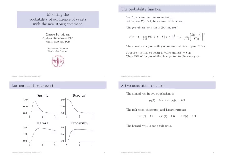
Log-normal time to event A two-population example The annual risk in two populations is Density Survival 1.0 1.0 g 0 ( t ) = 0 . 5 and g 1 ( t ) = 0 . 9 0.5 0.5 The risk ratio, odds ratio, and hazard ratio are 0.0 0.0 RR( t ) = 1 . 8 OR( t ) = 9 . 0 HR( t ) = 3 . 3 0 2 4 0 2 4 Hazard Probability The hazard ratio is not a risk ratio. 2.0 1.0 1.0 0.5 0.0 0.0 0 2 4 0 2 4 Stata Users Meeting, Stockholm, August 30, 2019 3 Stata Users Meeting, Stockholm, August 30, 2019 4

  2. The new stpreg command Proportional-odds models – Estimates virtually any probability function model Let x denote a covariate. We consider the proportional-odds model – Allows time-dependent effects g ( t | x ) g 0 ( t ) – Has postestimation commands (predict, test, lincom, estat, ...) 1 − g ( t | x ) = 1 − g 0 ( t ) exp( β 1 x ) – Stems from stgenreg by Crowther and Lambert (2013) The above can be written as logit g ( t | x ) = logit g 0 ( t ) + β 1 x Download it with The baseline function can be anything, e.g. . net from http://www.imm.ki.se/biostatistics/stata . net install stpreg logit g 0 ( t ) = θ 0 + θ 1 t logit g 0 ( t ) = θ 0 + θ 1 spline 1 ( t ) + θ 2 spline 2 ( t ) The quantity exp( β 1 ) is the odds ratio per unit-increase in x . Stata Users Meeting, Stockholm, August 30, 2019 5 Stata Users Meeting, Stockholm, August 30, 2019 6 Flexible proportional-odds model Predicted event probabilities We estimate a flexible proportional-odds model . predict predicted, probability . gen years = rectime/365.24 . qui webuse brcancer, clear . tw line predict years if x4a==0, sort || line predict years if x4a==1, sort . qui stset rectime, failure(censrec = 1) scale(3652.4) . stpreg x4a, df(2) nolog 1.0 Event-probability regression Number of obs = 686 Log likelihood = -667.42897 Odds Ratio Std. Err. z P>|z| [95% Conf. Interval] Probability x4a 5.082306 1.795635 4.60 0.000 2.542856 10.1578 0.5 _eq1_cp2_rcs1 1.415463 .1732414 2.84 0.005 1.113572 1.799197 _eq1_cp2_rcs2 2.369021 .3778431 5.41 0.000 1.733037 3.238395 _cons .7311249 .2436484 -0.94 0.347 .3804761 1.404933 Note: _cons estimates baseline odds. 0.0 The odds are 5.1 times greater in the larger tumor grade group. 0 3 6 Follow-up time (years) Stata Users Meeting, Stockholm, August 30, 2019 7 Stata Users Meeting, Stockholm, August 30, 2019 8

  3. Probability-power models Flexible probability-power model Let x denote a covariate. We estimate a flexible probability-power model We consider the probability-power model . stpreg x4a, power df(2) nolog Event-probability regression Number of obs = 686 g 0 ( t ) exp( β 1 x ) g ( t | x ) = ¯ ¯ Log likelihood = -668.30844 Power param. Std. Err. z P>|z| [95% Conf. Interval] where ¯ g ( t ) = 1 − g ( t ). x4a 2.584105 .6285316 3.90 0.000 1.604252 4.162439 _eq1_cp2_rcs1 1.207611 .0890262 2.56 0.011 1.045143 1.395335 The above can be written as _eq1_cp2_rcs2 1.692367 .1611357 5.53 0.000 1.404264 2.039577 _cons .5631365 .1349343 -2.40 0.017 .3520915 .9006827 log {− log[¯ g ( t | x )] } = log {− log[¯ g 0 ( t )] } + β 1 x The power parameter (hazard ratio) is 2.6. The baseline probability function ¯ g 0 ( t ) can be anything. The power parameter exp( β 1 ) is a measure of association. It corresponds to the hazard ratio per unit-increase in x . Stata Users Meeting, Stockholm, August 30, 2019 9 Stata Users Meeting, Stockholm, August 30, 2019 10 Semi-parametric probability-power model The probability and the hazard function We estimate a semi-parametric probability-power model The probability and the hazard functions are (Bottai, 2017) . stcox x4a, nolog noshow � 1 � S ( t + δ ) δ Cox regression -- Breslow method for ties 1 δ = 1 − lim g ( t ) = 1 − lim δ → 0 P ( T > t + δ | T > t ) No. of subjects = 686 Number of obs = 686 S ( t ) δ → 0 No. of failures = 299 � 1 � Time at risk = 211.2035922 δ → 0 P ( T ≤ t + δ | T > t )1 1 − S ( t + δ ) h ( t ) = lim δ = lim LR chi2(1) = 19.92 S ( t ) δ Log likelihood = -1778.2134 Prob > chi2 = 0.0000 δ → 0 _t Haz. Ratio Std. Err. z P>|z| [95% Conf. Interval] It can be shown that (Bottai, 2017) x4a 2.566048 .6241802 3.87 0.000 1.592993 4.133481 g ( t ) = 1 − exp[ − h ( t )] The power parameter (hazard ratio) is 2.6. The probability is always smaller than the hazard g ( t ) < h ( t ) Stata Users Meeting, Stockholm, August 30, 2019 11 Stata Users Meeting, Stockholm, August 30, 2019 12

  4. Conclusions References – Hazards are often mistaken for probabilities. Bottai, M. (2017). A regression method for modelling geometric rates. – For example, “the risk increases by 68% (HR = 1.68)” . Statistical Methods in Medical Research 26, 2700-2707. – This problem is consequential (Sutradhar & Austin, 2018). Bottai, M., Discacciati, A. and Santoni, G. (submitted). Modeling the probability of occurrence of events. – stpreg makes modeling probability functions simple. Crowther, M. and Lambert, P. (2013). stgenreg: A stata package for general parametric survival analysis. Journal of Statistical Software 53, 1-17. Discacciati, A. and Bottai, M. (2017). Instantaneous geometric rates via generalized linear models. Stata Journal 17, 358-371. Sutradhar, R. and Austin, P. C. (2018). Relative rates not relative risks: addressing a widespread misinterpretation of hazard ratios. Annals of Epidemiology 28, 54-57. Stata Users Meeting, Stockholm, August 30, 2019 13 Stata Users Meeting, Stockholm, August 30, 2019 14

Download Presentation
Download Policy: The content available on the website is offered to you 'AS IS' for your personal information and use only. It cannot be commercialized, licensed, or distributed on other websites without prior consent from the author. To download a presentation, simply click this link. If you encounter any difficulties during the download process, it's possible that the publisher has removed the file from their server.

Recommend


More recommend