The plan Intro: LOCAL model, synchronicity, Bellman- Ford Network - - PowerPoint PPT Presentation

Network Algorithms

Boaz Patt-Shamir Tel Aviv University

1

The plan

• Intro: LOCAL model, synchronicity, Bellman-

Ford

• Subdiameter algorithms: independent sets

and matchings

• CONGEST model: pipelining, more matching,

lower bounds

2

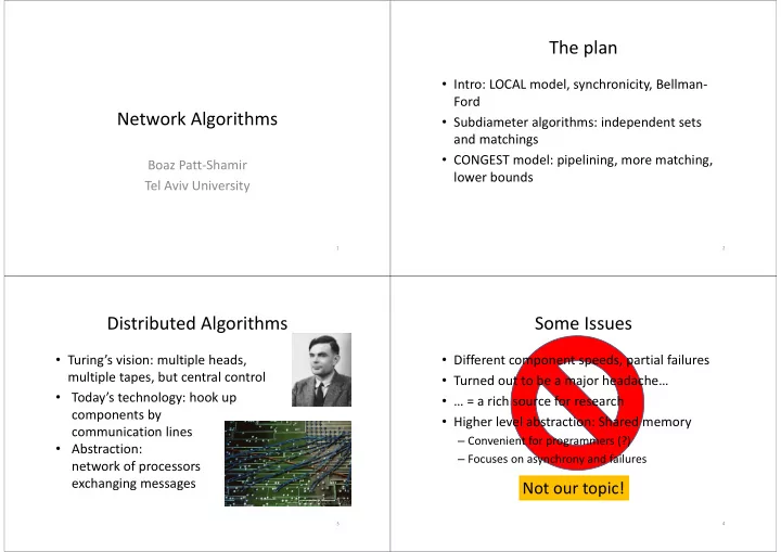
Distributed Algorithms

• Turing’s vision: multiple heads,

multiple tapes, but central control

3

• Today’s technology: hook up

components by communication lines

• Abstraction:

network of processors exchanging messages

Some Issues

• Different component speeds, partial failures
• Turned out to be a major headache…
• … = a rich source for research
• Higher level abstraction: Shared memory

– Convenient for programmers (?) – Focuses on asynchrony and failures

4

Not our topic!

Our Focus: Communication

The LOCAL model

• Connecvity ≡ a graph
• diameter =
• Nodes compute, send & receive msgs
• No failures (nodes or links)
• Running time:

– DEFINE: longest message delay ≡ one me unit – Neglect local processing time

5

The LOCAL model: Typical Tasks

• Compute functions of the topology

– Spanning Trees: Breadth-First (shortest paths), Minimum weight (MST) – Maximal Independent Set, Maximal Matching

• Communication tasks

– Broadcast, gossip, end-to-end

• In general: input/output relation

– Dynamic version: reactive tasks

6

The locality of distributed problems

A problem can be solved in time in LOCAL iff the following algorithm works:

• Each node collects full information from its
• neighborhood, and computes output

Time is the “radius” of input influence. LOCAL time = problem locality!

• Example:

lower bound on time for approx. MIS, Matching [KMW’06]

7

Example: Broadcast

• A source node has a message all nodes need

to learn

– Input: environment to source at time 0

• Protocol: When a new message received, send

to all neighbors (flooding)

• Time:
• Can be used to build a spanning tree:

– Mark edge delivering first message as parent

8

Example: Find maximum

• Each node has an input number from
• Want to find maximum
• Protocol: Whenever a new maximum

discovered, announce to all neighbors

• Time to convergence:
• #messages:
• Message size:

bits

9

Example: What’s ?

• Goal: find the number of nodes in the system
• Must assume some symmetry breaking

– exercise

• Standard assumption: Unique IDs from

– Usually assume

()

• Solution:

– Use a broadcast from each node

• Converge in

time

• #messages

10

Example: What’s ?

Another symmetry breaking tool: randomization Algorithm:

• 1. Each node

chooses a value

• 2. Find
• 3. Output .

Message length: . Can be off by a

• factor. Repeat and report

average to decrease variance.

11

Generic Algorithm

• 1. Each node broadcasts its input
• 2. Each node computes locally its output
• Time:

, #messages Can do better!

• 1. Build a single tree (how?)
• 2. Apply algorithm in tree
• #messages
• Time?

12

Asynchrony gives trouble

• A tree may grow quickly in a skewed way…

13

Asynchrony gives trouble

• A tree may grow quickly in a skewed way…

…But when used for the second time, we may pay for the skew!

14

The Bellman-Ford Algorithm

• Goal: Given a root, construct a shortest-paths

tree

• Protocol:

– every node maintains a variable – Root has always – Non-root sets

• Can show: stabilizes in time

15

The Bellman-Ford Algorithm

• Goal: Given a root, construct a shortest-paths

tree

• Protocol:

– every node maintains a variable – Root has always – Non-root sets

• Can show: stabilizes in time

16

B-F: Trouble With Asynchrony

Convergence in () time, but strange things can happen…

• Schedule : empty schedule
• Schedule :

1. Allow one message: from − − 1 to − on edge of weight 2 (incoming value: + 2) 2. Apply nodes to nodes − , … 3. Allow another message: from − − 1 to − on edge of weight 0 (incoming value: ) 4. Apply nodes to nodes − , …

2 2 2 2 1 1 2 4

• 17

B-F: Trouble With Asynchrony

Convergence in () time, but strange things can happen…

• Under schedule : node receives 2 distinct messages
• Node

receives messages in time units?!

2 2 2 2 1 1 2 4

• 18

Synchronous model

If all processors and links run in the same speed: Execution consists of rounds. In each round:

• 1. Receive messages from previous round

– Round 1: receive inputs

• 2. Do local computation
• 3. Send messages

Avoid skewed evolution!

19

Synchronous BFS tree construction

• Protocol: When first message received, mark
• rigin as parent and send to all neighbors

– Input: environment to source at time 0 – Break ties arbitrarily

• Natural uniform “ball growing” around origin
• Time:

20

Synchronizer

• Can emulate synchronous environment on

top of asynchronous one

• Abstraction: consistent pulse at all nodes

synchronizer

• asynch. netw.

msgs+

• synch. app.

msgs pulse

21

How:

• send a message to each

neighbor in each round (send null message if nothing to send)

• Emit pulse when received

messages from all neighbors

• synch. netw.

Therefore:

• Asynchronous networks are interesting only if

there may be faults

– Or when we care about #messages

• We henceforth assume synchronous

networks…

– But we need to account for messages!

22

Generic Synchronous Algorithm

• Any i/o-relation solvable in diameter time:

1. Construct a BFS tree

(need IDs/randomization to choose root: Leader Election!)

2. Send all inputs to root (“convergecast”) 3. Root computes all outputs, sends back (“broadcast”)

• Ridiculous? That’s the client-server model!

– Bread-and-butter distributed computing in the 70’s- 90’s, and beyond…

• Interesting? Theoretically : sub-diameter upper

and lower bounds

23

Subdiameter algorithms

24

Independent Sets

• Independent set (IS): a set of nodes, no

neighbors

• Maximum: terribly hard
• Maximal: cannot be extended

– Can be MUCH smaller than maximum IS

• Trivial sequentially!

– Linear time

• Can this parallelized?

25

Independent Sets

Turan’s theorem: There always exists an IS of size . [

is the average degree]

Proof: By the probabilistic method. Assign labels to nodes by a random permutation. Let be the nodes whose label is a local minimum. Lemma:

• . 

26

Lemma:

• .

Proof: By the Means Inequality.

• ()
• ∑
• . 

Lemma & Proof

∈

∈

27

Distributed MIS algorithm

• Each node chooses a random label

– Say, in

to avoid collisions w.h.p.

• Local minima enter MIS, neighbors eliminated
• Repeat.

Claim: In expectation, at least half of the edges are eliminated in a round.

28

Proof of Claim

Say node is killed by neighbor if is smallest in An edge is killed by node if is killed by . Observation: An edge can be killed by at most two nodes: the node with minimal label in and the node with minimal label in

• 29
• ().

Hence:

• ∈

∈ = 1 2 () + () + () () + ()

, ∈

• . 

Proof of Claim (cont.)

30

Distributed Matching

31

Definitions

• Input: Graph G=(V,E), with weights w : E→R+
• A matching: a set of disjoint edges
• Maximum cardinality matching (MCM)
• Maximum weighted matching (MWM)

32

Application: Switch Scheduling

input ports

• utput

ports

Goal: move packets from inputs to their outputs

33

Application: Switch Scheduling

Goal: move packets from inputs to their outputs At each time step, fabric can forward

– one packet from each input – one packet to each output

• To maximize throughput,

find MCM! fabric

input ports

• utput

ports

34

Note: Bipartite Graphs

• In many applications, nodes are

partitioned into two subsets (input/output, boys/girls)

• Bipartite graphs: = (1 ∪ 2, )

where

∩ = ∅ and ⊆ 1 × 2

• Matching is simpler in this case

– Bipartite MCM: max flow – bipartite MWM: min cost flow

V1 V2

35

Distributed Matching

Clearly, MCM must take diameter time!

• Information traverses the system: must decide

between the following alternatives

• r

36

MCM: Reduction to MIS

• Edge graph: If = (, ) then in

:

– The node set is – (, ’) are connected in () if they share a node in

• Observation:

is a matching in is independent in

b a f d e c b a f d e c

37

Approximate Distributed Matching

Theorem: Maximal matching is ½-approximate MCM. Proof: Let be a maximal matching, and

∗ an MCM.

Observe that

• 1. Any edge in

touches edges in

∗.

• 2. Any edge in

∗ touches

edge in . Map each edge in to the

∗ edges it touches.

By (1): #edges mapped to is at most . By (2), all MCM edges are mapped to, i.e.,

∗



38

• Basic concept: augmenting path for a matching M

– alternating M-edges and non-M edges – starts and ends with unmatched nodes

• Flipping membership in M increases the size of

matching Theorem: if all augmenting paths w.r.t. M have length at least 2k-1 then |M| (1-1/k) |MCM|

Augmenting Paths

39

MCM: Generic Approximation

Generic algorithm: input is G, ε M = ∅ For k=1 to 1/ε do Create “conflict graph” CG(k): nodes = augmenting paths of length 2k-1 edges = pairs of intersecting augmenting paths Find MIS in CG(k) Augment M by flipping edges of paths in MIS //well defined!

40

MCM: Generic Approximation

Why works? Hopcroft-Karp. Distributed implementation:

• 1. Nodes collect map of neighborhood to distance 2k+1
• 2. Appoint leader for each AP (say, endpoint with smaller ID)
• 3. Leaders simulate MIS algorithm of conflict graph

Complexity:

• Time: () rounds for (1 − 1/)-approximation
• Messages are large... (neighborhood to distance 2k+1)
• #paths is  much computation, even larger messages

41

Ergo: The CONGEST model

42

• Same as LOCAL, but

messages may contain up to bits

• Usually

– Allows messages to carry IDs and variables

• f magnitude
• – Similar to the “word model” in RAM

– Exact value of usually doesn’t matter

• Captures network algorithms more faithfully

Canonical Algorithm for CONGEST

Same algorithm:

• 1. Construct a BFS tree
• 2. Send all input to root
• 3. Root computes all outputs, sends back

Running time: . Why? In CONGEST, messages may be delayed!

• Pipelining…

43

Basic Pipelining

Theorem: Suppose messages travel on shortest paths. Then no message is delayed more than

• steps. (Any starting times!)
• Proof: Place a token on a message

. If it is delayed by and then meets again, let token take detour with .

44

route of route of ′ ′ delays , ′ meet

Basic Pipelining

45

Token not delayed ′ delays , ′ meet

Theorem: Suppose messages travel on shortest paths. Then no message is delayed more than

• steps. (Any starting times!)
• Proof: Place a token on a message

. If it is delayed by and then meets again, let token take detour with .

Proof (cont.)

• Before and after token’s detour:

– Same endpoints, same start time, same finish time – Same length (shortest paths!) – Hence same number of delays

• But the delay at switching point eliminated
• Consider a sequence of detours: the vector of

times-of-delay decreases lexicographically

• Hence if we repeatedly switch, process ends

46

Proof (end)

• Applying detour maintains #delays
• Eventually cannot apply detour:

– Recall: Detour applicable if token is delayed by and then meets again.

• If detour not applicable, no message delays

token twice

• Final message does not delay token at all.
• Hence #delays ≤ # other messages. 

47

Canonical Algorithm for CONGEST

Same algorithm:

• 1. Construct a BFS tree
• 2. Send all input to root
• 3. Root computes all outputs, sends back

Running time: . Why?

• In a tree, all paths are shortest, length

.

• Each piece of input is a message

48

Back to Matching

Generic algorithm: input is G, M = For k:=1 to

• do

Create “conflict graph” CG(k): nodes := augmenting paths of length 2k-1 edges := pairs of intersecting augmenting paths Find MIS in CG(k) Augment M by flipping edges of paths in MIS //well

defined!

49

Matching in CONGEST?

Recall MIS: random label per AP, local minima win Observations:

• Leader can select its own local winner
• Winner can be constructed rather than discovered
• All that’s needed is that each node knows how many

APs it belongs to And that’s easy in bipartite graphs!

50

Goal: count how many shortest APs of prescribed length end at gray nodes. Idea: BFS.

• start with unmatched white nodes (1)
• each node sums all first incoming numbers

– later messages ignored

• white nodes send sum to all neighbors
• gray nodes send sum to their mate
• last nodes know exactly how many APs end

with them

2 1 1 1 1 1 1 2 1 1 2 1 1 1 2 1 1 2 1 1 3 2 2 1 3 2 1 1 1 3 2 2 1 3 2 1 4 6 2

Counting APs in Bipartite Graphs

51

Goal: pick a uniformly random AP among all ending at a specific node. Idea: inductive construction.

• start at leader (bottom grey)
• at grey nodes, pick edge with probability

proportional to number on its far end

• at white nodes, follow matching edge

This defines a uniformly chosen random winner path for each leader. Remains: resolve conflicts between leaders.

2 1 1 1 1 1 1 2 1 1 2 1 1 1 2 1 1 2 1 1 3 2 2 1 3 2 1 1 1 3 2 2 1 3 2 1 4 6 2

Counting APs in Bipartite Graphs

52

Algorithm for Bipartite Graphs

• Count number of augmenting paths for each leader
• A leader of paths picks a number distributed like

the minimum of uniform variables (easy).

• Token selects next edge with probability proportional to

#paths that lead to that edge.

• Each node records the smallest it has seen
• After creating path, token backtracks unless killed
• best path joins MIS, etc.

53

Algorithm for Bipartite Graphs

• #nodes in conflict graph = #APs of length

– at most

/ .

• Hence

– Random labels have bits ( messages) – #iterations is

• Iteration

is emulated in steps

• Time complexity:
• for a given ,
• ver all since

.

54

General Graphs

• Idea: reduction to bipartite
• Means:

– Color nodes black or white randomly – Ignore monochromatic edges – Apply bipartite algorithm

• Can prove: Repeating / times suffice

(w.h.p.) Theorem: For any constant , in any graph,

• MCM can be computed distributively

in time ) using messages of size .

55

Lower Bounds

56

Bad Graphs for CONGEST

• Low diameter: there’s always a shortcut

– Good enough for LOCAL

• In CONGEST: when shortcuts are narrow, low

diameter not enough to transmit massive data

• State of the art: graphs of diameter

for problems that need to transport bits

– Extends to diameter 3 with weaker lower bounds

57

Bad Graphs for CONGEST: Basic Construction

• Bulk:

paths of length each

• Connect corresponding nodes by

a star

• Build a tree whose leaves are the

star centers => diameter File Transfer Problem: transmit bits from sender to receiver

• PR’99: Must take

) time!

sender receiver

58

Bad Graphs for CONGEST: Very small diameter [LPP’01,E’04]

• For

: replace binary tree with a d-ary tree, where

/().

Lower bound:

• For

: replace tree by a clique. Lower bound:

/

• How about

sender receiver

59

Bad Graphs for CONGEST: Applications

• To prove a time lower-bound on ,

reduce “file transfer” to :

– = MST (edge weights) [PR’99] – Stable Marriage (rankings) [KP’09]

• Strengthening: Can’t even

approximate MST

sender receiver

60

Conclusion

• Simple abstractions to model networks
• Some nice algorithmic techniques
• Many open problems

– Heterogeneous link bandwidth – Complexity of applications in low-diameter networks – Incorporating faults into model

61

Thanks!

62