The original problem Let X 1 , . . . , X n be a random sample from a - - PowerPoint PPT Presentation

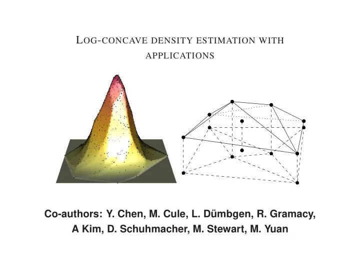
LOG-CONCAVE DENSITY ESTIMATION WITH

APPLICATIONS

Co-authors: Y. Chen, M. Cule, L. D¨ umbgen, R. Gramacy, A Kim, D. Schuhmacher, M. Stewart, M. Yuan

• R. J. Samworth

Log-concave densities

The original problem

Let X1, . . . , Xn be a random sample from a density f0 in Rd. How should we estimate f0? Two main alternatives:

• Parametric models: use e.g. MLE. Assumptions often

too restrictive.

• Nonparametric models: use e.g. kernel density
• estimate. Choice of bandwidth difficult, particularly

for d > 1.

June 3, 2013- 2

• R. J. Samworth

Log-concave densities

Shape-constrained estimation

Nonparametric shape constraints are becoming increasingly popular (Groeneboom et al. 2001, Walther 2002, Pal et al. 2007, D¨

umbgen and Rufibach 2009, Schuhmacher et al. 2011, Seregin and Wellner 2010, Koenker and Mizera 2010 . . .).

E.g. log-concavity, r-concavity, k-monotonicity, convexity. A density f is log-concave if log f is concave.

• Univariate examples: normal, logistic, Gumbel

densities, as well as Weibull, Gamma, Beta densities for certain parameter values.

June 3, 2013- 3

• R. J. Samworth

Log-concave densities

Characterising log-concave densities

Cule, S. and Stewart (2010)

Let X have density f in Rd. For a subspace V of Rd, let PV (x) denote the orthogonal projection of x onto V . Then in order that f be log-concave, it is:

• 1. necessary that for any subspace V , the marginal

density of PV (X) is log-concave (Pr´

ekopa 1973), and the

conditional density fX|PV (X)(·|t) of X given PV (X) = t is log-concave for each t

• 2. sufficient that, for every (d − 1)-dimensional

subspace V , the conditional density fX|PV (X)(·|t) of X given PV (X) = t is log-concave for each t.

June 3, 2013- 4

• R. J. Samworth

Log-concave densities

Unbounded likelihood!

Consider maximising the likelihood L(f) = n

i=1 f(Xi)

• ver all densities f.

June 3, 2013- 5

• R. J. Samworth

Log-concave densities

Existence and uniqueness

Walther (2002), Cule, S. and Stewart (2010)

Let X1, . . . , Xn be independent with density f0 in Rd, and suppose that n ≥ d + 1. Then, with probability one, a log-concave maximum likelihood estimator ˆ fn exists and is unique.

June 3, 2013- 6

• R. J. Samworth

Log-concave densities

Sketch of proof

Consider maximising over all log-concave functions ψn(f) = 1 n

n

• i=1

log f(Xi) −

• Rd f(x) dx.

Any maximiser ˆ fn must satisfy:

• 1. ˆ

fn(x) > 0 iff x ∈ Cn ≡ conv(X1, . . . , Xn)

• 2. Fix y = (y1, . . . , yn) and let ¯

hy : Rd → R be the smallest concave function with ¯ hy(Xi) ≥ yi for all i. Then log ˆ fn = ¯ hy∗ for some y∗ 3.

• Rd ˆ

fn(x) dx = 1.

June 3, 2013- 7

• R. J. Samworth

Log-concave densities

Schematic diagram of MLE on log scale

June 3, 2013- 8

• R. J. Samworth

Log-concave densities

Computation

Cule, S. and Stewart (2010), Cule, Gramacy and S. (2009)

First attempt: minimise τ(y) = − 1 n

n

• i=1

¯ hy(Xi) +

• Cn

exp{¯ hy(x)} dx.

June 3, 2013- 9

• R. J. Samworth

Log-concave densities

Computation

Cule, S. and Stewart (2010), Cule, Gramacy and S. (2009)

First attempt: minimise τ(y) = − 1 n

n

• i=1

¯ hy(Xi) +

• Cn

exp{¯ hy(x)} dx. Better: minimise σ(y) = − 1 n

n

• i=1

yi +

• Cn

exp{¯ hy(x)} dx. Then σ has a unique minimum at y∗, say, log ˆ fn = ¯ hy∗ and σ is convex . . .

June 3, 2013- 10

• R. J. Samworth

Log-concave densities

Computation

Cule, S. and Stewart (2010), Cule, Gramacy and S. (2009)

First attempt: minimise τ(y) = − 1 n

n

• i=1

¯ hy(Xi) +

• Cn

exp{¯ hy(x)} dx. Better: minimise σ(y) = − 1 n

n

• i=1

yi +

• Cn

exp{¯ hy(x)} dx. Then σ has a unique minimum at y∗, say, log ˆ fn = ¯ hy∗ and σ is convex . . . but non-differentiable!

June 3, 2013- 11

• R. J. Samworth

Log-concave densities

Log-concave projections

Let Pk be the set of probability distributions P on Rk with

• Rk x dP(x) < ∞ and P(H) < 1 for all hyperplanes H.

Let Fk be the set of upper semi-continuous log-concave densities on Rk. The condition P ∈ Pd is necessary and sufficient for the existence of a unique log-concave projection ψ∗ : Pd → Fd given by ψ∗(P) = argmax

f∈Fd

• Rd log f dP.

(Cule, S. and Stewart, 2010; Cule and S., 2010; D¨ umbgen, S., Schuhmacher, 2011). June 3, 2013- 12

• R. J. Samworth

Log-concave densities

One-dimensional characterisation

D¨ umbgen, S. and Schuhmacher (2011)

Let P0 ∈ P1 have distribution function F0. Let S(f∗) = {x ∈ R : log f∗(x) > 1

2 log f∗(x−δ)+ 1 2 log f∗(x+δ) ∀δ > 0}.

Then the distribution function F ∗ of f∗ is characterised by x

−∞

{F ∗(t) − F0(t)} dt    ≤ 0 for all x ∈ R = 0 for all x ∈ S(f∗) ∪ {∞}.

June 3, 2013- 13

• R. J. Samworth

Log-concave densities

Example 1

Suppose f0(x) = 1

2(1 + x2)−3/2. Then f∗(x) = 1 2e−|x|.

June 3, 2013- 14

• R. J. Samworth

Log-concave densities

Example 2

June 3, 2013- 15

• R. J. Samworth

Log-concave densities

Log-concave projections preserve independence Chen and S. (2012)

Suppose P ∈ Pd can be written as P = P1 ⊗ P2, where P1 and P2 are probability measures on Rd1 and Rd2, with d2 = d − d1. If f∗ is the log-concave projection of P and f∗

ℓ is the projection of Pℓ (ℓ = 1, 2), then

f∗(x) = f∗

1 (x1)f∗ 2 (x2)

for x = (xT

1 , xT 2 )T ∈ Rd.

This makes log-concave projections very attractive for independent component analysis (S. and Yuan, 2012).

June 3, 2013- 16

• R. J. Samworth

Log-concave densities

Convergence of log-concave densities

Cule and S. (2010), Kim and S. (2013)

Let (fn) be a sequence of u.s.c. log-concave densities on Rd with corresponding probability measures (νn) satisfying νn

d

→ ν. If dim

• csupp(ν)
• = d, then

(a) ν is absolutely continuous w.r.t. Lebesgue measure

• n Rd, with log-concave Radon–Nikodym derivative

f = cl(lim inf fn). (b) Let a0 > 0 and b0 ∈ R be such that f(x) ≤ e−a0x+b0. If a < a0 then

• eax|fn(x) − f(x)| dx → 0 and, if f is

continuous, supx eax|fn(x) − f(x)| → 0.

June 3, 2013- 17

• R. J. Samworth

Log-concave densities

Theoretical properties

Cule and S. (2010), D¨ umbgen, S. and Schuhmacher (2011)

The log-concave projection is continuous with respect to Wasserstein (Mallows-1) distance. In particular, let X1, . . . , Xn

iid

∼ P0 ∈ Pd, and let f∗ = ψ∗(P0). Taking a0 > 0 and b0 ∈ R such that f∗(x) ≤ e−a0x+b0, we have for any a < a0 that

• Rd eax| ˆ

fn(x) − f∗(x)| dx a.s. → 0, and, if f∗ is continuous, supx eax| ˆ fn(x) − f∗(x)| a.s. → 0.

June 3, 2013- 18

• R. J. Samworth

Log-concave densities

Global minimax bounds

Kim and S. (2013)

We have inf

˜ fn

sup

f∈Fd

E

• Rd( ˜

fn − f)2

• ≥

d 560 × 25(d+1)(d+4)/(2d) n−4/(d+4). Similar lower bounds (with different constants) hold for L2

1, Hellinger, Kullback–Leibler, chi-squared losses.

Under a growth condition on − log f, we can obtain the same rates up to logarithmic factors for a Bayesian predictive estimator (Yang and Barron, 1999). When d ≤ 4, the log-concave MLE attains these rates for fixed f.

June 3, 2013- 19

• R. J. Samworth

Log-concave densities

Moment (in)equalities

D¨ umbgen, S. and Schuhmacher (2011)

Let P ∈ Pd, let f∗ = ψ∗(P) and let P ∗(B) =

• B f∗. Then
• Rd x dP ∗(x) =
• Rd x dP(x)

and

• Rd h dP ∗ ≤
• Rd h dP

for all convex h : Rd → (−∞, ∞].

June 3, 2013- 20

• R. J. Samworth

Log-concave densities

Smoothed log-concave density estimator

D¨ umbgen and Rufibach (2009), Cule, S. and Stewart (2010), Chen and S. (2012)

Let ˜ fn = ˆ fn ∗ φ ˆ

A,

where φ ˆ

A is a d-dimensional normal density with mean

zero and covariance matrix ˆ A = ˆ Σ − ˜ Σ. Here, ˆ Σ is the sample covariance matrix and ˜ Σ is the covariance matrix corresponding to ˆ fn. Then ˜ fn is a smooth, fully automatic log-concave estimator supported on the whole of Rd which satisfies the same theoretical properties as ˆ fn. It offers potential improvements for small sample sizes.

June 3, 2013- 21

• R. J. Samworth

Log-concave densities

Breast cancer data

June 3, 2013- 22

• R. J. Samworth

Log-concave densities

Classification boundaries

June 3, 2013- 23

• R. J. Samworth

Log-concave densities

Testing for log-concavity Chen and S. (2012)

Suppose P0 ∈ Pd and let A∗ denote the difference between the covariance matrix of P0 and that of its log-concave projection. Then A∗ = 0 if and only if P0 has a log-concave density. We can therefore use tr( ˆ A) as a test statistic, and generate a critical value from bootstrap samples drawn from ˆ fn. This test is consistent: if P0 is not log-concave, then the power converges to 1 as n → ∞.

June 3, 2013- 24

• R. J. Samworth

Log-concave densities

Regression problems

D¨ umbgen, S. and Schuhmacher (2011)

Consider the regression model Yi = µ(xi) + ǫi, i = 1, . . . , n, where ǫ1, . . . , ǫn are i.i.d., log-concave and E(ǫi) = 0. In both of the cases i) µ is linear and ii) µ is isotonic, we can jointly estimate µ and the distribution of ǫi. Significant improvements are obtainable over usual methods when errors are non-normal.

June 3, 2013- 25

• R. J. Samworth

Log-concave densities

ICA models

Comon (1994)

In the simplest, noiseless case of ICA, we observe replicates x1, . . . , xn of X

d×1 = A d×d S d×1,

where the mixing matrix A is invertible and S has independent components. Our main aim is to estimate the unmixing matrix W = A−1; estimation of marginals P1, . . . , Pd of S = (S1, . . . , Sd) is a secondary goal. This semiparametric model is therefore related to PCA.

June 3, 2013- 26

• R. J. Samworth

Log-concave densities

Different previous approaches

• Postulate parametric family for marginals P1, . . . , Pd;
• ptimise contrast function involving (W, P1, . . . , Pd).

Contrast usually represents mutual information or maximum entropy; or non-Gaussianity (Eriksson et al., 2000,

Karvanen et al., 2000).

• Postulate smooth (log) densities for marginals (Bach and

Jordan, 2002; Hastie and Tibshirani, 2003; Samarov and Tsybakov, 2004, Chen and Bickel, 2006). June 3, 2013- 27

• R. J. Samworth

Log-concave densities

Our approach

• S. and Yuan (2012)

To avoid assumptions of existence of densities, and choice of tuning parameters, we propose to maximise the log-likelihood ℓn(W, f1, . . . , fd) = log | det W| + 1 n

n

• i=1

d

• j=1

log fj(wT

j xi)

• ver all d × d non-singular matrices W = (w1, . . . , wd)T,

and univariate log-concave densities f1, . . . , fd. To understand how this works, we need to understand log-concave ICA projections.

June 3, 2013- 28

• R. J. Samworth

Log-concave densities

ICA notation

Let W be the set of d × d invertible matrices. The ICA model PICA

d

consists of those P ∈ Pd with P(B) =

d

• j=1

Pj(wT

j B),

∀ Borel B, for some W ∈ W and P1, . . . , Pd ∈ P1. The log-concave ICA model FICA

d

consists of f ∈ Fd with f(x) = | det W|

d

• j=1

fj(wT

j x) with W ∈ W, f1, . . . , fd ∈ F1.

If X has density f ∈ FICA

d

, then wT

j X has density fj.

June 3, 2013- 29

• R. J. Samworth

Log-concave densities

Log-concave ICA projections

Let ψ∗∗(P) = argmax

f∈FICA

d

• Rd log f dP.

We also write L∗∗(P) = supf∈FICA

d

• Rd log f dP.

The condition P ∈ Pd is necessary and sufficient for L∗∗(P) ∈ R and then ψ∗∗(P) defines a non-empty, proper subset of FICA

d

.

June 3, 2013- 30

• R. J. Samworth

Log-concave densities

An example

Suppose P is the uniform distribution on the unit Euclidean disk in R2. Then ψ∗∗(P) includes all f ∈ FICA

d

that can be represented by an arbitrary orthogonal W ∈ W and f1(x) = f2(x) = 2 π(1 − x2)1/2

June 3, 2013- 31

• R. J. Samworth

Log-concave densities

Schematic picture of maps

Pd

ψ∗

− → Fd

ψ∗∗

ց PICA

d ψ∗∗|PICA

d

− → FICA

d

June 3, 2013- 32

• R. J. Samworth

Log-concave densities

Log-concave ICA projection on PICA

d

If P ∈ PICA

d

, then ψ∗∗(P) defines a unique element of FICA

d

. The map ψ∗∗|PICA

d

coincides with ψ∗|PICA

d

. Moreover, suppose that P ∈ PICA

d

, so that P(B) =

d

• j=1

Pj(wT

j B),

∀ Borel B, for some W ∈ W and P1, . . . , Pd ∈ P1. Then f∗∗(x) := ψ∗∗(P)(x) = | det W|

d

• j=1

f∗

j (wT j x),

where f∗

j = ψ∗(Pj).

June 3, 2013- 33

• R. J. Samworth

Log-concave densities

Identifiability

Comon (1994), Eriksson and Koivunen (2004)

Suppose a probability measure P on Rd satisfies P(B) =

d

• j=1

Pj(wT

j B) = d

• j=1

˜ Pj( ˜ wT

j B)

∀ Borel B, where W, ˜ W ∈ W and P1, . . . , Pd, ˜ P1, . . . , ˜ Pd are probability measures on R. Then there exists a permutation π and scaling vector ǫ ∈ (R \ {0})d such that ˜ Pj(Bj) = Pπ(j)(ǫjBj) and ˜ wj = ǫ−1

j wπ(j) iff none of P1, . . . , Pd is a Dirac mass

and not more than one of them is Gaussian. Consequence: If P ∈ PICA

d

, then ψ∗∗(P) is identifiable iff P is identifiable.

June 3, 2013- 34

• R. J. Samworth

Log-concave densities

Consistency

Suppose P 0 is identifiable. For any maximiser ( ˆ W n, ˆ fn

1 , . . . , ˆ

fn

d ) of ℓn(W, f1, . . . , fd), there exist ˆ

πn ∈ Πd and ˆ ǫn

1, . . . , ˆ

ǫn

d ∈ R \ {0} such that

(ˆ ǫn

j )−1 ˆ

wn

ˆ πn(j) a.s.

→ w0

j and

∞

−∞

• |ˆ

ǫn

j | ˆ

fn

ˆ πn(j)(ˆ

ǫn

j x)−f∗ j (x)

• dx a.s.

→ 0, for j = 1, . . . , d, where f∗

j = ψ∗(P 0 j ).

June 3, 2013- 35

• R. J. Samworth

Log-concave densities

Pre-whitening

Pre-whitening is a standard pre-processing step in ICA algorithms to improve stability. We replace the data with z1 = ˆ Σ−1/2x1, . . . , zn = ˆ Σ−1/2xn, and maximise the log-likelihood over O ∈ O(d) and g1, . . . , gd ∈ F1. If ( ˆ On, ˆ gn

1 , . . . , ˆ

gn

d ) is a maximiser, we then set

ˆ ˆ W n = ˆ On ˆ Σ−1/2 and ˆ ˆ fn

j = ˆ

gn

j .

Thus to estimate the d2 parameters of W 0, we first estimate the d(d + 1)/2 free parameters of Σ, then maximise over the d(d − 1)/2 free parameters of O.

June 3, 2013- 36

• R. J. Samworth

Log-concave densities

Equivalence of pre-whitened algorithm

Suppose P 0 is identifiable and

• Rd x2 dP 0(x) < ∞. With

probability 1 for large n, a maximiser ( ˆ ˆ W n, ˆ ˆ fn

1 , . . . , ˆ

ˆ fn

d ) of

ℓn(W, f1, . . . , fd) over W ∈ O(d)ˆ Σ−1/2 and f1, . . . , fd ∈ F1

• exists. For any such maximiser, there exist ˆ

ˆ πn ∈ Πd and ˆ ˆ ǫn

1, . . . , ˆ

ˆ ǫn

d ∈ R \ {0} such that

(ˆ ˆ ǫn

j )−1 ˆ

ˆ wn

ˆ ˆ πn(j) a.s.

→ w0

j

and ∞

−∞

• |ˆ

ˆ ǫn

j | ˆ

ˆ fn

ˆ ˆ πn(j)(ˆ

ˆ ǫn

j x)−f∗ j (x)

• dx a.s.

→ 0, where f∗

j = ψ∗(P 0 j ).

June 3, 2013- 37

• R. J. Samworth

Log-concave densities

Computational algorithm

With (pre-whitened) data x1, . . . , xn, consider maximising ℓn(W, f1, . . . , fd)

• ver W ∈ O(d) and f1, . . . , fd ∈ F1.

(1) Initialise W according to Haar measure on O(d) (2) For j = 1, . . . , d, update fj with the log-concave MLE

• f wT

j x1, . . . , wT j xn (D¨

umbgen and Rufibach, 2011)

(3) Update W using projected gradient step (4) Repeat (2) and (3) until negligible relative change in log-likelihood.

June 3, 2013- 38

• R. J. Samworth

Log-concave densities

Exp(1)-1

−4 −2 2 4 6 −2 −1 1 2 3 4

Truth

S1 S2 −4 −2 2 4 6 −2 −1 1 2 3 4

Rotated

X1 X2 −4 −2 2 4 6 −2 −1 1 2 3 4

Reconstructed

S ^

1

S ^

2

−1 1 2 3 4 5 0.0 0.2 0.4 0.6 0.8 1.0 s Marginal Densities

June 3, 2013- 39

• R. J. Samworth

Log-concave densities

0.7N(−0.9, 1) + 0.3N(2.1, 1)

−6 −4 −2 2 4 6 −4 −2 2 4

Truth

S1 S2 −6 −4 −2 2 4 6 −4 −2 2 4

Rotated

X1 X2 −6 −4 −2 2 4 6 −4 −2 2 4

Reconstructed

S ^

1

S ^

2

−4 −2 2 4 0.00 0.10 0.20 0.30 s Marginal Densities

June 3, 2013- 40

• R. J. Samworth

Log-concave densities

Performance comparison

LogConICA FastICA ProDenICA 0.0 0.2 0.4 0.6 0.8 1.0

Uniform

Amari Metric LogConICA FastICA ProDenICA 0.0 0.2 0.4 0.6 0.8 1.0

Exponential

Amari Metric LogConICA FastICA ProDenICA 0.0 0.2 0.4 0.6 0.8 1.0

t2

Amari Metric LogConICA FastICA ProDenICA 0.0 0.2 0.4 0.6 0.8

Mixture of Normal

Amari Metric LogConICA FastICA ProDenICA 0.0 0.2 0.4 0.6 0.8 1.0

Binomial

Amari Metric

June 3, 2013- 41

• R. J. Samworth

Log-concave densities

Summary

• The log-concave MLE is a fully automatic,

nonparametric density estimator

• It has several extensions which can be used in a wide

variety of applications, e.g. classification, clustering, functional estimation, regression and Independent Component Analysis problems.

• Many challenges remain: faster algorithms, dependent

data, further theoretical results, other applications and constraints,...

June 3, 2013- 42

• R. J. Samworth

Log-concave densities

References

• Bach, F., Jordan, M. I. (2002) Kernel independent component analysis. Journal of Machine Learning

Research, 3, 1–48.

• Balabdaoui, F., Rufibach, K. and Wellner, J. A. (2009), Limit distribution theory for maximum

likelihood estimation of a log-concave density, Ann. Statist., 37, 1299–1331.

• Chen, A. and Bickel, P. J. (2006) Efficient independent component analysis, The Annals of Statistics,

34, 2825–2855.

• Chen, Y. and Samworth, R. J. (2012), Smoothed log-concave maximum likelihood estimation with

applications, Statist. Sinica, to appear.

• Comon, P. (1994) Independent component analysis, A new concept? Signal Proc., 36, 287–314.
• Cule, M., Gramacy, R. and Samworth, R. (2009) LogConcDEAD: an R package for maximum

likelihood estimation of a multivariate log-concave density, J. Statist. Software, 29, Issue 2.

• Cule, M. and Samworth, R. (2010), Theoretical properties of the log-concave maximum likelihood

estimator of a multidimensional density. Electron. J. Statist., 4, 254–270.

• Cule, M., Samworth, R. and Stewart, M. (2010), Maximum likelihood estimation of a multi-dimensional

log-concave density. J. Roy. Statist. Soc., Ser. B. (with discussion), 72, 545–607.

• D¨

umbgen, L. and Rufibach, K. (2009) Maximum likelihood estimation of a log-concave density and its distribution function: Basic properties and uniform consistency. Bernoulli, 15, 40–68. June 3, 2013- 43

• R. J. Samworth

Log-concave densities

• D¨

umbgen, L., Samworth, R. and Schuhmacher, D. (2011), Approximation by log-concave distributions with applications to regression. Ann. Statist., 39, 702–730.

• Eriksson, J. and Koivunen, V. (2004) Identifiability, separability and uniqueness of linear ICA models.

IEEE Signal Processing Letters, 11, 601–604.

• Groeneboom, P., Jongbloed, G. and Wellner, J. A. (2001) Estimation of a convex function:

Characterizations and asymptotic theory. Ann. Statist., 29, 1653–1698.

• Hastie, T. and Tibshirani, R. (2003) Independent component analysis through product density
• estimation. In Advances in Neural Information Processing Systems 15 (Becker, S. and

Obermayer, K., eds), MIT Press, Cambridge, MA. pp 649–656.

• Kim, A. and Samworth, R. J. (2013) Global minimax bounds for log-concave density estimation. In

preparation.

• Koenker, R. and Mizera, I. (2010) Quasi-concave density estimation. Ann. Statist., 38, 2998–3027.
• Pal, J., Woodroofe, M. and Meyer, M. (2007) Estimating a Polya frequency function. In Complex

datasets and Inverse problems, Networks and Beyond Tomography, vol. 54 of Lecture Notes - Monograph Series, 239–249. IMS.

• Pr´

ekopa, A. (1973) On logarithmically concave measures and functions. Acta Scientarium Mathematicarum, 34, 335–343.

• Samarov, A. and Tsybakov, A. (2004), Nonparametric independent component analysis. Bernoulli, 10,

565–582.

• Samworth, R. J. and Yuan, M. (2012) Independent component analysis via nonparametric maximum

likelihood estimation, Ann. Statist., to appear. June 3, 2013- 44

• R. J. Samworth

Log-concave densities

• Schuhmacher, D., H¨

usler, A. and D¨ umbgen, L. (2011) Multivariate log-concave distributions as a nearly parametric model. Statistics & Risk Modeling, 28, 277–295.

• Seregin, A. and Wellner, J. A. (2010) Nonparametric estimation of convex-transformed densities.
• Ann. Statist., 38, 3751–3781.
• Walther, G. (2002) Detecting the presence of mixing with multiscale maximum likelihood. J. Amer.
• Statist. Assoc., 97, 508–513.
• Yang, Y. and Barron, A. (1999) Information-theoretic determination of minimax rates of convergence.
• Ann. Statist., 27, 1564–1599.

June 3, 2013- 45