The objective function (for two consecutive slices) is as follows: - - PowerPoint PPT Presentation

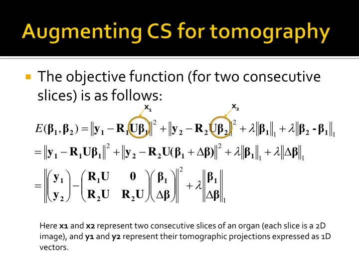
 The objective function (for two consecutive

slices) is as follows:

1 2 1 1 2 2 1 1 2 2

) , ( β β β β U R U R U R y y β β β) U(β R y Uβ R y β

• β

β Uβ R y Uβ R y β β

1 1 2 2 1 2 1 1 1 2 2 1 1 1 1 2 1 2 2 2 1 1 1 2 1

                                                 E

x1 x2 Here x1 and x2 represent two consecutive slices of an organ (each slice is a 2D image), and y1 and y2 represent their tomographic projections expressed as 1D vectors.

 The previous algorithms for tomographic

reconstruction assumed that the angles of Radon projection were accurately known.

 In certain applications, this assumption is

surprisingly invalid.

 This is called as “tomography under unknown

angles”.

 Application 1: Patient motion during CT

scanning

 Application 2: Moving insect tomography  Application 3: Cryo-electron tomography

 Application 3: Cryo-electron tomography  In this, one collects multiple (nearly) identical

samples of a structure (such as a virus) which we wish to image.

 Each slide contains thousands of virus particles

(i.e. samples) packed in a substrate such as ice.

 A tomographic projection is obtained by passing

an electron-ray beam through all particles, through some angle.

 The electron beam usually destroys the sample, and hence

another tomographic projection of a different sample (containing virus particles of the same type) is acquired.

 The problem is that each virus particle will be oriented

randomly, and all the orientations are unknown!

 To make matters worse, the low power of the electron

beam produces measurements that are extremely noisy.

 In such applications, however several hundred or even

thousand projections (all under unknown angles) are acquired.

https://en.wikipedia.org/wiki/Cryogenic_electron_ microscopy

Ajit Rajwade

https://med.nyu.edu/skirball

• lab/stokeslab/phi12.html

Ajit Rajwade

https://ki.se/en/research/core-facility-for-electron-tomography-0

 Particle picking from noisy micrographs  In some algorithms, similar particles are

clustered and averaged to reduce noise

 Given the series of particle images, we then

seek to solve jointly for the angles of projection and the underlying structure

Ajit Rajwade

 Nobel in Chemistry in 2017  More details here below:

https://www.nobelprize.org/nobel_prizes/chemistry/laureates/ 2017/advanced-chemistryprize2017.pdf

Ajit Rajwade

 Moment-based approach  Ordering-based approach  Approach using dimensionality reduction

(similar to ordering-based approach).

 We shall restrict ourselves to 2D images and

1D tomographic projections although the theory is extensible to 3D images (and their 2D projections)

 The moment of order (p,q) of an image f(x,y)

is defined as follows:

 The moment of order (p,q) where k=p+q of an

image f(x,y) is defined as follows:

 Note that there can exist multiple pairs of

(p,q) which sum up to k, and these are all called order k image moments.

 The order n moment of a tomographic

projection at angle θ is defined as follows:

 Substituting the definition of Pθ(s) into Mθ(n):

 Using the binomial theorem, we have:  We will use this to derive a neat relationship

between the tomographic projection moments and the image moments!

 See next slide.

Image moment of order (n-l,l)

Substituting n = 0, with measurements at one angle. Substituting n = 1, with measurements at two angles.

Substituting n = k, with measurements at k+1 different angles.

These equations are called the Helgason- Ludwig consistency conditions (HLCC), and they give relations between image and projection moments. One can prove that the matrix A is invertible if and only if the projections are acquired at k+1 distinct angles. In fact, unique k+1 angles are necessary and sufficient for estimation of the image moments of order 0 through to order k.

 In the tomography under unknown angles

problem, we would know neither the image moments nor the angles of acquisition.

 In such a case, the underlying image can be

• btained only up to an unknown rotation.

 To understand why, see the next slide.

θ1 θ2 θ3 In the first case you took projections of an object at three angles θ1, θ2, θ3 +θ1 + θ2 + θ3 In the second case you took projections of a version of the same

• bject but rotated by  at three

angles  +θ1,  +θ2,  +θ3 In both cases, the projections will be identical! The parameter  will always be indeterminate – but this is not a problem in most applications

Image source: Malhotra and Rajwade, “Tomographic reconstruction with unknown view angles exploiting moment-based relationships”

https://www.cse.iitb.ac.i n/~ajitvr/eeshan_icip201 6.pdf

 Given tomographic projections of a 2D image in 8 or more

distinct and unknown angles, the image moments of order 1 and 2, as well as the angles can be uniquely recovered – but up to the aforementioned rotation ambiguity.

 This result is true for almost any 2D image (i.e. barring a set of

very rare “corner case” images).

 This result was proved in 2000 by Basu and Bresler at UIUC in a

classic paper called “Uniqueness of tomography with unknown view angles”.

 In an accompanying paper called “Feasibility of tomography

with unknown view angles”, they also proved that these estimates are stable under noise.

 The proof of the theorem and the discussion of the corner cases

is outside the scope of our course.

 In other words, systems of equations of the

following form have a unique solution in the angles and the image moments, but modulo the rotation ambiguity:

n n l l n i l n l i l n n

IM A M l n C PM

i i

) ( , ) (

sin cos ) , (



 



 

  



Image moments Projection moments Column vector of image moments of

• rder n

This is the n-th row of a matrix and it represents the linear combination coefficients for moments of

• rder n and at angle θi.

 We can now build an algorithm for the

aforementioned problem.

 Minimize the following objective function in

an alternating fashion:

 Start with a random initial angle estimate and

compute the image moments by matrix inversion.

 



  

 

N n Q i n n n Q i i

IM A PM IM E

i i

1 2 ) ( ) ( 1)

} { , (







 Next, do an independent brute force search over

each angle θi. * For every value of θi sampled from 0 to 180, determine the image moments using that value, and hence determine the value of E. * Choose the value of θi corresponding to the least value of E.

 Perform a multi-start strategy for the best

possible results – since this cost function is highly nonconvex.

 Remember: these angles can be estimated

• nly up to a global angular offset  which is

indeterminate.

 Following the angle estimates, the underlying

image can be reconstructed using FBP.