The Maple computer algebra environment In the presentation that - - PDF document

> >

• >

> > > (3) (3) (2) (2) (4) (4)

• (1)

(1)

• >

> > >

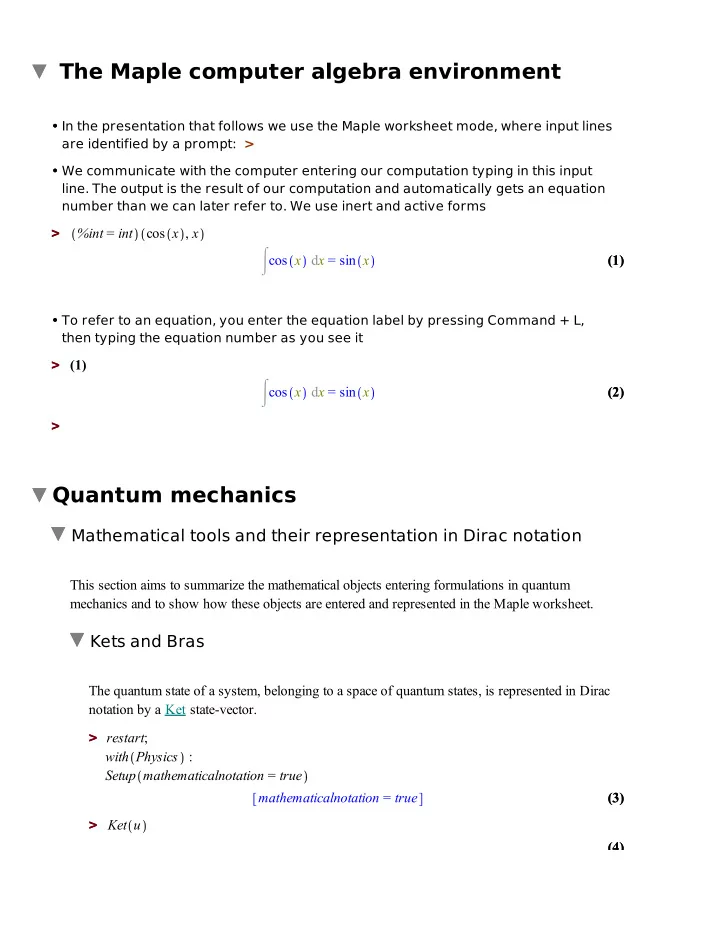
The Maple computer algebra environment

In the presentation that follows we use the Maple worksheet mode, where input lines are identified by a prompt: > We communicate with the computer entering our computation typing in this input

• line. The output is the result of our computation and automatically gets an equation

number than we can later refer to. We use inert and active forms

%int = int cos x , x cos x dx = sin x

To refer to an equation, you enter the equation label by pressing Command + L, then typing the equation number as you see it

(1) cos x dx = sin x

Quantum mechanics

Mathematical tools and their representation in Dirac notation

This section aims to summarize the mathematical objects entering formulations in quantum mechanics and to show how these objects are entered and represented in the Maple worksheet.

Kets and Bras

The quantum state of a system, belonging to a space of quantum states, is represented in Dirac notation by a Ket state-vector. restart; with Physics : Setup mathematicalnotation = true mathematicalnotation = true Ket u

> > > > > > (7) (7) (6) (6) (5) (5) (4) (4) (8) (8) > > > > (9) (9) (10) (10) > > u The above is the quantum analog of a non-projected vector u of a 3-D Euclidean space. The norm of a generic Ket u is not predefined and can be indicated by setting a bracket rule, as shown below. Every Ket can be projected onto a basis of state-vectors of the space to which the Ket belongs. The Kets conforming a basis (analogous to 3-D unit vectors) are distinguished from a generic Ket u by the fact that they have one or many quantum numbers, as in Ket v, n vn Kets having quantum numbers are always assumed to belong to a basis of quantum states, are

• rthogonal to each other, have norm equal to 1, and are distinguished from each other by the

values of these quantum numbers. For example, an orthonormal basis of a two dimensional space of quantum states is Ket v, 0 , Ket v, 1 v0 , v1 There are no restrictions on the number of quantum numbers that a Ket can have. This is a Ket belonging to a basis of a space that depends on four quantum numbers. Ket v, j, k, m, n vj, k, m, n You can associate a space of states with each quantum number, so a Ket with many quantum numbers represents a state in a space constructed as a tensor product of spaces. There is a Bra associated with each Ket, obtained from the Ket by performing the Hermitian conjugate, or Dagger, operation. Dagger % vj, k, m, n Dagger % vj, k, m, n You can enter Bras directly by using the Bra function. Bra v, j, k, m, n vj, k, m, n The space of Bras of a system is the dual of the space of Kets of that system.

(15) (15) > > > > > > (12) (12) > > (13) (13) > > (17) (17) (14) (14) > > (11) (11) (16) (16) > >

Discrete and continuous basis of states

Kets belong to either a discrete or a continuous spaces of quantum states. A discrete space of states is one where the quantum numbers of its Kets vary discretely. These Kets thus belong to discrete bases of quantum states. A continuous space is one where the quantum numbers vary continuously and its Kets belong to continuous bases of quantum states. Unless explicitly stated

• therwise, Kets are assumed to belong to discrete space of states.

You can indicate that a label R identifies a continuous space of states by using the Setup command. Setup continuous = R * Partial match of 'continuous' against keyword 'quantumcontinuousbasis' quantumcontinuousbasis = R Kets of a continuous space of states can also have any number of quantum numbers. Ket R, x Rx Ket R, x, y, z Rx, y, z Dagger % Rx, y, z

Scalar product and orthonormalization relation

The scalar product is defined between a Bra and a Ket, in that order, and can be performed by using the dot operator `.` of the Physics package, or by using the Bracket function; both represent the same object. Bra u . Ket v u v Bracket Bra u , Ket v u v Note that when the scalar product is just represented, not actually computed, as in the above, the result is always expressed in terms of the Bracket function. A shortcut notation for entering the scalar product using the Bracket function is Bracket u, v

(18) (18) > > (17) (17) (22) (22) > > (23) (23) > > (24) (24) (19) (19) > > (21) (21) > > > > (20) (20) > > u v Under the Dagger operation, A B † = B† A† so that the Bracket becomes Dagger % v u For the Bracket, the same happens under conjugation: conjugate % u v Two generic Kets such as the above may or not belong to the same space. To make practical use

• f Kets, depending on the problem you may want to set a bracket rule, stating the value of the

Bracket between them, by using the Setup command. Setup % = f u, v bracketrules = u v = f u, v After that, both the dot operator of the Physics package and the Bracket function know how to perform their scalar product. Bracket u, v f u, v Kets belonging to a discrete basis of states satisfy an orthonormalization relation involving the KroneckerDelta symbol, and when the quantum numbers are present, you do not need to specify a bracket rule. %Bracket Bra u, n , Ket u, m = Bra u, n . Ket u, m un um =

m, n

Note in the above the inert form %Bracket. It is sometimes useful to represent mathematical

• perations without having them actually performed. For that purpose, use any command with the

name prefixed by the symbol %. To have the inert operation performed, use the value command. value %

m, n = m, n

Evaluate the the output two operations above at m = n. eval (22), m = n un un = 1 The Bracket of state-vectors depending on many quantum numbers results in products of KroneckerDelta symbols. The shortcut notation of the Bracket function also works in the presence of quantum numbers (tip: to avoid typographical mistakes, it is practical to group the

(26) (26) (30) (30) > > > > > > (28) (28) (29) (29) > > (25) (25) > > (27) (27) > >

• bjects visually, by leaving spaces or not after the commas).

Bracket u, i, j, k, u, n, m, l ;

i, n j, m k, l

Kets of a continuous basis of states satisfy an orthonormalization relation involving the Dirac function (recall that R has been set as a label of a continuous space, by using the Setup command, above). Bracket R, x, R, y y x %Bracket R, x, y, z, R, a, b, c : % = value % Rx, y, z Ra, b, c =

3

a x, b y, c z In the above, the 3-dimensional Dirac function can be expanded using expand expand (27) Rx, y, z Ra, b, c = a x b y c z

Closure relation, Projectors

Every Ket of a space of states can be expanded into a basis of that space. The operator that performs the expansion is called a Projector. To construct these projectors, information about the basis dimension is necessary. You can indicate this dimension directly to the Projector command, or set it by using Setup. The information available at this point is Setup basisdim, cont * Partial match of 'basisdim' against keyword 'quantumbasisdimension' * Partial match of 'cont' against keyword 'quantumcontinuousbasis' quantumbasisdimension = none, quantumcontinuousbasis = R By default, continuous bases are assumed to range from to , so this information on R is enough to compute its Projector. P R Projector Ket R, x, y, z PR Rx, y, z Rx, y, z dx dy dz This expression PR for the projector is also called the closure relation; together with the

• rthonormalization relation

Rx, y, z Ra, b, c =

3

a x, b y, c z , it tells that the set of Kets Rx, y, z containing all the possible values of x, y, and z forms a basis, and so

> > > > (34) (34) (36) (36) > > > > (31) (31) (32) (32) (33) (33) > > > > > > (37) (37) (38) (38) > > (35) (35) any has a unique expansion onto Rx, y, z . Note that the scalar product of PR with itself is equal to itself. P R . P R Rx, y, z Rx, y, z dx dy dz The following is the projector for a basis generically labeled u that has not been set to represent a continuous basis. By default, if nothing is known about the label of a basis, it is assumed to be related to a discrete space of states. The dimension of the basis can be indicated directly to the Projector command. P u Projector Ket u, n , dimension = N Pu

n = 0 N 1

un un The information passed to Projector is automatically tracked by the system, so you do not need to give it again. Setup quantumbasisdimension, quantumcontinuousbasis quantumbasisdimension = R = , u = N , quantumcontinuousbasis = R To change this information, see Setup and its redo option. In order to compute scalar products

• f Kets belonging to a basis with other Kets of the same space, you can define a bracketrule.

%Bracket Bra R, x, y, z , Ket psi = psi x, y, z Rx, y, z = x, y, z Setup % bracketrules = u v = f u, v , Rx, y, z = x, y, z Now Bracket and the `.` operator of the Physics package know how to compute a number of related operations. Bracket Bra R, a, b, c , Ket psi a, b, c P R . Ket psi x, y, z Rx, y, z dx dy dz Bra psi . P R

> > > > > > > > (45) (45) > > (40) (40) (44) (44) (43) (43) (42) (42) > > > > (39) (39) (38) (38) (41) (41) x, y, z Rx, y, z dx dy dz Bra psi . P R . Ket psi x, y, z

2 dx dy dz

This is a bracket rule for the scalar product of a state-vector of the discrete basis u and . %Bracket Bra u, n , Ket psi = psi n un = n Setup % bracketrules = u v = f u, v , Rx, y, z = x, y, z , un = n This rule for un permits projecting

• nto the u basis, which is equivalent to

inserting a projector between and . Note the use of delay evaluation quotes surrounding the Bracket; the operation is performed in the next line by using %. ' Bracket psi, P u , psi ' Pu %

n = 0 N 1

n

2

A Ket can have different types of spaces associated with its quantum numbers. In the following example, Kets from a basis B have four quantum numbers, two of which, B3 and B4, are associated with continuous spaces, and the dimension of the space associated with each quantum number is different. Setup quantumcontinuousbasis = B 3 , B 4 , quantumbasisdimension = B 1 = 1 /2 ..1 /2, B 2 = 0 ..N, B 3 = a ..a, B 4 = infinity ..infinity quantumbasisdimension = R = , u = N, B1 = 1 2 .. 1 2 , B2 = 0 ..N, B3 = a ..a, B4 = .. , quantumcontinuousbasis = R, B3, B4 This is the projector onto the basis B: Projector Ket B, n, m, x, y

> > (48) (48) (45) (45) > > > > (47) (47) (49) (49) (46) (46) (50) (50) > > > >

a a m = 0 N n = 0 1

B

n 1 2 , m, x, y

B

n 1 2 , m, x, y

dx dy

Quantum operators, eigenvectors, eigenvalues and commutators

To indicate to the system that a letter represents a quantum operator, use the

Setup command; this sets B as a quantum operator. Setup op = B * Partial match of 'op' against keyword 'quantumoperators' quantumoperators = B Note that after having entered Setup mathematicalnotation = true the extended typesetting displays noncommutative objects in different colors; to change this color, see ?Setup. Because B is now a quantum operator, Bm, n, x, y is an eigenvector of the four operators B1, B2, B3, and B4, with eigenvalues m, n, x, and y, respectively. For example, B 2 . Ket B, m, n, x, y n Bm, n, x, y

Quantum operators can also be 3-D Euclidean vectors; for that purpose, you must load the Physics[Vectors] subpackage.

with Vectors &x, ` `, `.`, ChangeBasis, ChangeCoordinates, Component, Curl, DirectionalDiff, Divergence, Gradient, Identify, Laplacian, , Norm, Setup, diff Set the vectors L, r , and p as quantum operators (note the use of the option redo to erase previous definitions of quantum operators). Setup op = L_, r_, p_, x, y, z, px, py, pz, Lx, Ly, Lz , redo * Partial match of 'op' against keyword 'quantumoperators' quantumoperators = L, Lx, Ly, Lz, p, px, py, pz, r, x, y, z Define L as the angular momentum operator L = r p, and set commutation rules for the components of r and p. L_ r_ &x p_ L r p

(56) (56) (53) (53) (51) (51) > > > > (54) (54) (55) (55) > > (52) (52) > > > > > > r_ x _i y _j z _k r i x j y k z p_ px _i py _j pz _k; p i px j py k pz Vector calculus with noncommutative components preserves A B = B A and A B = B

• A. This is achieved by symmetrizing and antisymmetrizing, respectively, each of

these products. For example, below is the Component of L along the x-axis. _i . L_ y pz z py To enter the commutation rules between each component of r and p with each other, you can write these commutators and pass the whole set to Setup. When there are many, as in this case, it is more convenient to use a Matrix and an indexing function. Enter the core information as a procedure: C represents the Commutator of the Components of the vectors a and b. C a_, i, b_, j %Commutator Component a_, i , Component b_, j C a, i, b, j a i, b j So, given i and j from 1 to 3 identifying the components of r and p, an algebra can be set as set as follows. algebra i, j C r_, i, p_, j = I * KroneckerDelta i, j , C r_, i, r_, j = 0, C p_, i, p_, j = 0 algebra i, j C r, i, p, j = I i, j, C r, i, r, j = 0, C p, i, p, j = 0 Now all of the commutators between each component of r and p can be constructed with one call to Matrix. Matrix 3, 3, algebra x, px = I, x, x = 0, px, px = 0, x, py = 0, x, y = 0, px, py = 0, x, pz = 0, x, z = 0, px, pz = 0 , , y, px = 0, y, x = 0, py, px = 0, y, py = I, y, y = 0, py, py = 0, y, pz = 0, y, z = 0, py, pz = 0 , , z, px = 0, z, x = 0, pz, px = 0, z, py = 0, z, y = 0, pz, py = 0, z, pz = I, z, z = 0, pz, pz = 0 ,

(61) (61) (59) (59) > > (63) (63) > > > > (64) (64) > > > > (62) (62) > > (58) (58) > > (60) (60) > > (57) (57) Pass this Matrix to Setup to set the algebra rules. Setup % algebrarules = px, py = 0, px, pz = 0, py, pz = 0, x, px = I, x, py = 0, x, pz = 0, x, y = 0, x, z = 0, y, px = 0, y, py = I, y, pz = 0, y, z = 0, z, px = 0, z, py = 0, z, pz = I , Set, for instance, the values of Lx, Ly, and Lz, the components of L. Lx _i . L_ Lx y pz z py Ly _j . L_ Ly z px x pz Lz _k . L_ Lz x py y px Verify the commutator algebra for these components of L. Commutator Lx, Ly = I Lz I y px I x py = I x py y px Commutator Lz, Lx = I Ly I x pz I z px = I z px x pz Commutator Ly, Lz = I Lx I z py I y pz = I y pz z py

The three equations above are identically true. Other operators frequently used in different contexts are the Annihilation and

Creation operators: they augment or diminish the value of a quantum number by

• ne. These operators are suitable, for instance, for working with multi-particle

vector states; in that context the quantum numbers are called occupation

• numbers. This constructs a pair of annihilation/creation operators acting on the

basis A involving only one quantum number.

am Annihilation A am a

(67) (67) > > (73) (73) > > (75) (75) > > > > > > > > (66) (66) (68) (68) (69) (69) (72) (72) > > > > (71) (71) > > (74) (74) (70) (70) (65) (65) > > > > ap Creation A ap a Annihilation and Creation operators act on Kets belonging to discrete bases and assume that the "lower" state happens when the quantum number is equal to zero (frequently called "vacuum": a ket with occupation number equal to zero represents a state with "no particles"). am . Ket A, n n An

1

am . % n n 1 An

2

ap . Ket A, n n 1 An

1

ap . % n 1 n 2 An

2

The Commutator of the operators a- and a are automatically set when these operators are constructed, and satisfy (note the use of the inert form %Commutator): %Commutator am, ap a , a value % 1 To indicate that the Kets of a basis are fermionic, use an anticommutative variable to label the

• basis. To set the prefix identifier of anticommutative variables use the Setup command.

Setup anticommutativeprefix = Theta anticommutativeprefix = , _ type Theta, anticommutative true Ket Theta Construct Annihilation and Creation operators acting on this basis; use the option notation = explicit so that the basis and the quantum numbers onto which these operators act are explicit. Am Annihilation Theta, notation = explicit Am a

1

> > (78) (78) (77) (77) (76) (76) > >

• >

> > > > >

• (79)

(79) > > (80) (80) (81) (81) > > > > (83) (83) > > (82) (82) Ap Creation Theta, notation = explicit Ap a

1

The AntiCommutator of these operators satisfy %AntiCommutator Am, Ap a

1

, a

1

value % 1 According to Pauli's exclusion principle, only one fermionic particle can be in a given state, so starting from the vacuum, Ket Theta, 0 Ap . %

1

Ap . % Am . %% And as is always the case, the annihilation operator acting on the vacuum returns zero Am . %

* Unitary Operators in Quantum Mechanics

* Eigenvalues of an unitary operator and exponential of Hermitian

• perators

Show that the eigenvalues of an unitary operator are all on the unit circle, their modulus is 1. Show that an operator ei H is unitary provided that H is Hermitian (H = H†) and is any real parameter. Solution

restart; with Physics : interface imaginaryunit = i :

(87) (87) > > (85) (85) > > (88) (88) > > > > > > (91) (91) (84) (84) (90) (90) (86) (86) > > (92) (92) > > > > (89) (89) > > > > Setup unitaryoperators = U unitaryoperators = U If U is a normalized eigenvector of U with eigenvalue U Ket U, = U Ket U, U U = U Dagger (85) U U† = U So, to show that the eigenvalues have modulus equal to 1, multiplying sides by sides (86) . (85) 1 =

2

To show that, when H is Hermitian, then V = ei H is unitary, Setup quantumoperators = V , hermitianoperators = H , realobjects = hermitianoperators = H , quantumoperators = H, U, V , realobjects = V = exp i H V = ei H Dagger (89) V† = e

i H

Again multiply sides by sides (89) . (90) V V† = 1 (90) . (89) V† V = 1 Therefore, V is unitary * Properties of unitary operators Consider two set of kets an and bn , each of them constituting a complete orthonormal basis of the same space.

(95) (95) (93) (93) (94) (94) > > > > (97) (97) (98) (98) > > (96) (96) > > > > > > > > > >

*Verify that U =

k = 0

bk ak , maps one basis into the other, i.e.: bn = U an restart; with Physics : Tell the system that an and bn , are complete orthonormal basis Setup quantumoperators = U , bracketrules = %Bracket Bra a, m , Ket a, n = KroneckerDelta m, n , %Bracket Bra b, m , Ket b, n = KroneckerDelta m, n bracketrules = am an =

m, n,

bm bn =

m, n , quantumoperators =

U U =

k = 0

Ket b, k Bra a, k U =

k = 0

bk ak Apply this operatorial equation to am '% . Ket a, m ' U =

k = 0

bk ak am % U am = bm

*Show that U =

k = 0

bk ak is unitary Recalling the expansion of the operator U (94) U =

k = 0

bk ak Dagger (94) U† =

k = 0

ak bk

(104) (104) > > > > (105) (105) (106) (106) (100) (100) > > > > > > > > (99) (99) (101) (101) > > > > (102) (102) (103) (103) > > Again multiply sides by sides '(98) . (94)' U† =

k = 0

ak bk U =

k = 0

bk ak % U† U =

k1 = 0

ak1 ak1 (94) . (98) U U† =

k1 = 0

bk1 bk1 and since an and bn form two complete basis of the same space, the right-hand sides are equal to the identity operator , and so U is unitary.

*Show that the matrix elements of U in the an and bn basis are equal

Recalling the expansion of the operator U (94) U =

k = 0

bk ak Compute now the matrix elements of U in the an and bn basis 'Bra a, n . (94) . Ket a, m ' an U =

k = 0

bk ak am % an U am = an bm Likewise 'Bra b, n . (94) . Ket b, m ' bn U =

k = 0

bk ak bm %

> > > > (106) (106) (109) (109) > > > > (107) (107) (108) (108) > > bn U bm = an bm Schrödinger equation and unitary transform Consider a ket

t that solves the time-dependant Schrödinger equation:

i t

t

= H t

t

and consider t = U t

t ,

where U t is a unitary operator. Does t evolves according a Schrödinger equation i t t = t t and if yes, which is the expression of t ?

Solution

restart; with Physics : interface imaginaryunit = i : Setup automaticsimplification = true, mathematicalnotation = true, quantumoperators = , hermitianoperators = H , unitaryoperators = U , realobjects = t, automaticsimplification = true, hermitianoperators = H , mathematicalnotation = true, quantumoperators = , H, U , realobjects = , t , unitaryoperators = U CompactDisplay U, H, t U t will now be displayed as U H t will now be displayed as H t will now be displayed as Ket , t = U t Ket , t

> > (116) (116) > > > > > > (112) (112) (117) (117) > > > > (109) (109) > > (113) (113) > > (114) (114) (118) (118) > > (110) (110) (115) (115) (111) (111)

t

= U

t

Compute now the evolution of t i diff (109), t i

t t = i Ut t

U

t t

Simplify this equation taking into account Schrödinger's equation for : i t Ket , t = H t Ket , t i

t t = H t

simplify (110), (111) , t Ket , t i

t t = i Ut t

U H

t

Now, from (109)

t

= U

t

U t * rhs = lhs (109) U† U

t

= U†

t

simplify (114)

t

= U†

t

Inserting this result in (112) subs (115), (112) i

t t = i Ut U† t

U H U†

t

the amiltonian for t is given by the coefficient of

t

• n the right-hand side

t = Coefficients rhs (116) , Ket , t = i Ut U† U H U† So

t

satisfies a Schrodinger equation and as one can expect, is Hermitian Dagger (117) (117)

(125) (125) (121) (121) (124) (124) > > (120) (120) (119) (119) > > (123) (123) > > (118) (118) > > > > > > > > (122) (122) > > > >

†

= i U U†

t

U† U H i Ut U† U H U† Recalling that U t satisfies U t U t * = U t U t * U U† = 1 diff (119), t Ut U† U U†

t = 0

subs (120), (118)

†

= i U U†

t

U† U H i Ut U† U H U† In the time independent case, i.e. U t = U, reduced to: U = U subs U t = U, (117) = i Ut U† U H U† % = U H U† Translation operators using Dirac notation In this section, we focus on the operator Ta = e

i a P

Settings

restart; with Physics : interface imaginaryunit = i : Setup realobjects = a, x, , m, x1, x2 , unitaryoperators = T , hermitianoperators = , X, P , quantumcontinuousbasis = X, P hermitianoperators = , P, X , quantumcontinuousbasis = P, X , realobjects = , a, m, x, x1, x2 , unitaryoperators = T Setup bracketrules = Bracket Bra P, p , Ket = p , Bracket Bra X, x ,

> > (127) (127) > > (126) (126) > > > > (132) (132) (128) (128) > > > > (129) (129) (131) (131) (130) (130) > > Ket = x , Bracket Bra X, x , Ket P, p = 2

1 2 exp

i x p bracketrules = Pp = p , Xx = x , Xx Pp = 2 e

i x p

2 Assume :: 0, Useful closure relations 1 = Projector Ket X, x 1 = Xx Xx dx To have equivalent projectors with different integration variables, we use as the identity

• perator:

1 = , 1 = 2 :

1 = Projector Ket P, p , 2 = Projector Ket P, q

1 =

Pp Pp dp, 2 = Pq Pq dq

The Action (translation) of the operator Ta = e

i a P

• n a ket

Considering a general ket , introduce a closure relation Ket =

1 Ket

=

1

subs (129), % = Pp Pp dp Bra X, x . %

> > (136) (136) > > > > (137) (137) > > (133) (133) > > (132) (132) (134) (134) > > (135) (135) x = 2 1 e

i x p

p 2 dp Which gives after a variable change x = y a PDEtools:-dchange x = y a, %, y , known = : subs y = x, % x a = 2 1 e

i x a p

p 2 dp Let's now evaluate the action of e

i a P

• n in the X, x basis

(131) = Pp Pp dp Bra X, x . e

i a P

. % Xx e

i a P

= 2 1 e

i p a x

p 2 dp Comparing the above with (133) % (133) Xx e

i a P

x a = 2 1 e

i p a x

p 2 dp 2 1 e

i x a p

p 2 dp simplify (136) Xx e

i a P

x a = 0 isolate %, x a

> > (145) (145) (144) (144) (142) (142) (141) (141) (143) (143) (138) (138) (140) (140) > > > > (139) (139) > > > > > > > > > > x a = Xx e

i a P

Action of Ta on an operator V X

Let's consider an operator V X , that can be written as a formal power series: V x =

n = 0

vn xn. Its matrix elements are: %Bracket = Bracket Bra X, x1 , V X , Ket X, x2 Xx1 V X Xx2 = V x2 x2 x1 Using the closure relation (128) 1 = Xx Xx dx V X can also be represented in the X, x basis as V X (128) V X = V x Xx Xx dx Let's now introduce two closure relations to evaluate V X in the momentum basis P Ket X, x =

1 Ket X, x , Bra X, x = Bra X, x 2

Xx =

1 Xx ,

Xx = Xx 2 subs %, (141) V X = V x 1 Xx Xx 2 dx Recalling (129)

1 =

Pp Pp dp, 2 = Pq Pq dq subs %, %% V X = V x Pp Pp dp Xx Xx Pq Pq dq dx

(150) (150) > > (152) (152) (146) (146) (148) (148) > > > > > > > > > > > > (147) (147) (151) (151) (149) (149) > > combine (145) V X = V x Pp Pp Xx Xx Pq Pq dq dp dx eval %, `*` = `.` V X = V x e

i x p q

Pp Pq 2 dq dp dx Apply now the translation operator Ta T a = exp i a P Ta = e

i a P

% . (147) . %* Ta V X Ta

† =

V x Pp Pq e

i p q a x

2 dq dp dx Making a variable change x = y a PDEtools:-dchange x = y a, %, y , known = V : subs y = x, % Ta V X Ta

† =

V x a Pp Pq e

i x p q

2 dq dp dx Evaluate the matrix element of this result and compute the integral Bra X, x1 % Ket X, x2 Xx1 Ta V X Ta

† Xx2

= V x a e

i x x1 p i x x2 q

4

2 2

dq dp dx value % Xx1 Ta V X Ta

† Xx2

= V x1 a x1 x2

(158) (158) > > > > (157) (157) > > (154) (154) > > > > (155) (155) > > (156) (156) > > > > (153) (153)

* The quantum operator components of L satisfy Lj, Lk = i j, k, m Lm

restart; with Physics : interface imaginaryunit = i : Setup spaceindices = lowercaselatin, automaticsimplification = true ; automaticsimplification = true, spaceindices = lowercaselatin

Define L, r and p as tensors of the 3-D Euclidean space embedded in

Define L, r, p Defined objects with tensor properties L, p, r, , , , g , ,

a, b, , , , , ,

Now set L, p, r as quantum operators and the related Commutator rules for the algebra in tensor notation

Setup quantumoperators = L, p, r , %Commutator p j , p k = 0, %Commutator r j , p k = i KroneckerDelta j, k , %Commutator r j , r k = 0 algebrarules = pj, pk = 0, rj, pk = i j, k, rj, rk = 0 , quantumoperators = L, p, r ,

The definition of Lj

L j = LeviCivita j, k, m r k p m Lj = rk pm j

k, m

The rule to be verified: %Commutator L j , L k = i LeviCivita j, k, m L m Lj, Lk = i j, k, m L m Substitute now the operator Li by its tensor form in terms rk and pm in the commutator above Library:-SubstituteTensor (156), (157) ra pm j

a, m, rb pc k b, c

= i j, k, m ra pb

a, b, m

Simplify, all in one go, we expect an identity Simplify (158)

> > > > > > > > > > (161) (161) (159) (159) (160) (160) i rj pk rk pj = i rj pk rk pj The same one step at a time, first expand the commutator on the left-hand side expand (158)

j a, m k b, c ra pm rb pc

rb pc ra pm = i j, k, m ra pb

a, b, m

Simplify (160) i rj pk rk pj = i rj pk rk pj

* Quantum Commutation Rules Basics, F X , p = i F X

Derive the commutation rules, in the coordinates representation, between an arbitrary function of the coordinates and the related momentum, departing from the differential representation pn = i n This exercise illustrate how to have full control of the computational process by using different elements of the Maple language, including inert representations of abstract vectorial differential

• perators, Hermitian operators, algebra rules, etc. It also illustrate the ability to perform

computations algebraically, using the product operator, but with differential operators, and transform the products into the application of the operators only when we want that, as we do with paper and pencil.

Solution

restart : with Physics : with Physics Vectors : interface imaginaryunit = i :

Set the problem:

all of x, y, z, px, py, pz are Hermitian operators all of x, y, z commute between each other

tell the system only that the operators x, y, z are the differentiation variables

• f the corresponding (differential) operators px, py, pz but do not tell what is the

form of the operators Setup differentialoperators = p_, x, y, z , hermitianoperators = p, x, y, z , algebrarules = %Commutator x, y = 0, %Commutator x, z = 0, %Commutator y, z

> > > > (167) (167) > > > > (164) (164) (166) (166) > > (162) (162) (165) (165) > > (163) (163) = 0 , quiet algebrarules = x, y = 0, x, z = 0, y, z = 0 , differentialoperators = p, x, y, z , hermitianoperators = p, x, y, z , Assuming F X is a smooth function, the idea is to apply the commutator F X , p to an arbitrary ket of the Hilbert space

x, y, z

, perform the operation explicitly after setting a differential operator representation for p, and from there get the commutation rule between F X and p. Start introducing the commutator, to proceed with full control of the operations we use the inert form %Commutator alias X = x, y, z : CompactDisplay F X F X will now be displayed as F %Commutator F X , p_ Ket , X F, p

x, y, z

This product of a commutator, involving a differential operator and and a function of the coordinates, and a Ket that depends on the coodinates, can be transformed into the (traditional in computer algebra) application of the differential operator when desired, as follows: (164) = Library:-ApplyProductsOfDifferentialOperators (164) F, p

x, y, z

= F p

x, y, z

p F

x, y, z

Note that, in p F X

x, y, z

, the application of p is not expanded: at this point nothing is known about p , it is not necessarily a linear operator. In the Quantum Mechanics problem at hands, however, it is. So give now the operator p an explicit representation as a linear vectorial differential operator (we use the inert form %Nabla, , to be able to proceed with full control

• ne step at a time)

p_ f i %Nabla f p f i f The expression (165) becomes (165) F, p

x, y, z

= i F

x, y, z

i F

x, y, z

Activate now the inert operator and simplify taking into account the algebra rules for the

(173) (173) > > (169) (169) (168) (168) > > > > > > > > > > (172) (172) > > (171) (171) > > (170) (170) coordinate operators x, y = 0, x, z = 0, y, z = 0 value (167) F, p

x, y, z

= i F

x, y, z x i x, y, z y j x, y, z z k

i Fx

x, y, z

, F

x, y, z x i

Fy

x, y, z

F

x, y, z y j

Fz

x, y, z

F

x, y, z z k

Simplify (168) F, p

x, y, z

= i i Fx

x, y, z

i j Fy

x, y, z

i k Fz

x, y, z

To make explicit the gradient in disguise on the right-hand side, factor out the arbitrary ket

x, y, z

Factor (169) F, p

x, y, z

= i Fx i Fy j Fz k

x, y, z

Combine now the expanded gradient into its inert (not-expanded) form Gradient = %Gradient F X Fx i Fy j Fz k = F subs (171), (170) F, p

x, y, z

= i F

x, y, z

Since (172) is true for all

x, y, z

, this ket can be removed from both sides of the equation. One can do that either taking coefficients (see Coefficients) or multiplying by the "formal inverse" of this ket, arriving at the (expected) form of the commutation rule between F X and p (172) Inverse Ket , x, y, z F, p = i F

Schrödinger vs Heisenberg picture

Within the Schrödinger picture of Quantum Mechanics, the time evolution of the state of a system, represented by a Ket t , is determined by Schrödinger's equation:

> > > > (174) (174) > > i d dt

t

= H

t

where H, the Hamiltonian, as well as the quantum operators OS representing observable quantities, are all time-independent. Within the Heisenberg picture, a Ket representing the state of the system does not evolve with time, but the operators OH t representing observable quantities, and through them the Hamiltonian H, do. Problem: Departing from Schrödinger's equation, a) Show that the expected value of a physical observable in Schrödinger's and Heisenberg's representations is the same, i.e. that

t OS t

= OH t b) Show that the evolution equation of an observable OH in Heisenberg's picture, equivalent to Schrödinger's equation, is given by: OH . t = i OH t , H where in the right-hand-side we see the commutator of OH with the Hamiltonian of the system.

Solution

Let OS and OH respectively be operators representing one and the same observable quantity in Schrödinger's and Heisenberg's pictures, and H be the operator representing the Hamiltonian of a physical system. All of these operators are Hermitian. So we start by setting up the framework for this problem accordingly, including that the time t and Planck's constant are real. To automatically combine powers of the same base (happening frequently in what follows) we also set combinepowersofsamebase = true. with Physics : interface imaginaryunit = i : Setup hermitianoperators = H, OH, OS , realobjects = t, , combinepowersofsamebase = true, mathematicalnotation = true combinepowersofsamebase = true, hermitianoperators = H, OH, OS, p, x, y, z , mathematicalnotation = true, realobjects = , i, j, k, , r, , , , r, , t, , x, y,

> > (176) (176) > > (179) (179) > > > > (177) (177) > > > > (175) (175) (180) (180) (178) (178) z Let's consider Schrödinger's equation i diff Ket , t , t = H Ket , t i

t t = H t

Now, H is time-independent, so (175) can be formally solved: t is obtained from the solution 0 at time t = 0, as follows: T exp i H t T e

i t H

Ket , t = T Ket , 0

t

= e

i t H

To check that (177) is a solution of (175), substitute it in (175): eval (175), (177) H e

i t H

= H e

i t H

Next, to relate the Schrödinger and Heisenberg representations of an Hermitian operator O representing an observable physical quantity, recall that the value expected for this quantity at time t during a measurement is given by the mean value of the corresponding operator (i.e., bracketing it with the state of the system

t

). So let OS be an observable in the Schrödinger picture: its mean value is obtained by bracketing the operator with equation (177): Dagger (177) OS (177)

t OS t

=

0 e i t H

OS e

i t H

The composed operator within the bracket on the right-hand-side is the operator O in Heisenberg's picture, OH t : Dagger T OS T = OH t e

i t H

OS e

i t H

= OH t Analogously, inverting this equation,

> > (183) (183) > > (182) (182) (181) (181) > > (185) (185) (184) (184) > > > > T (180) Dagger T OS = e

i t H

OH t e

i t H

As an aside to the problem, we note from these two equations, and since the operator T = e

i t H

is unitary (because H is Hermitian), that the switch between Schrödinger's and Heisenberg's pictures is accomplished through a unitary transformation. Inserting now this value of OS from (181) in the right-hand-side of (179), we get the answer to item a) lhs (179) = eval rhs (179) , (181)

t OS t

=

0 OH t

where, on the left-hand-side, the Ket representing the state of the system is evolving with time (Schrödinger's picture), while on the the right-hand-side the Ket

0 is constant and it is OH t ,

the operator representing an observable physical quantity, that evolves with time (Heisenberg picture). As expected, both pictures result in the same expected value for the physical quantity represented by O. To complete item b), the derivation of the evolution equation for OH t , we take the time derivative of the equation (180): diff rhs = lhs (180) , t OHt = i H e

i t H

OS e

i t H

i e

i t H

OS H e

i t H

To rewrite this equation in terms of the commutator OS, H , it suffices to re-order the product H e

i t H

in the first term, placing the exponential first: Library:-SortProducts (183), e

i t H

, H , usecommutator OHt = i e

i t H

H OS e

i t H

i e

i t H

H OS OS, H e

i t H

Normal (184)

> > > > (185) (185) (187) (187) > > > > > > (188) (188) (186) (186) OHt = i e

i t H

OS, H e

i t H

Finally, to express the right-hand-side in terms of OH t , H instead of OS, H , we take the commutator of the equation (181) with the Hamiltonian (181) OS = e

i t H

OH t e

i t H

Commutator (181), H OS, H = e

i t H

OH t , H e

i t H

Combining these two expressions, we arrive at the expected result for b), the evolution equation

• f a given observable OH in Heisenberg's picture

eval (185), (187) OHt = i OH t , H

Quantization of the energy of a particle in a magnetic field

Show that the energy of a particle of charge q and mass m in a constant magnetic field B oriented along the z axis can be written as H =

c a†a

1 2 where a†and a are creation and annihilation operators and

c = q B

m

Solution

The classical Hamiltonian is given by

> > > > > > > > (190) (190) (192) (192) (191) (191) (189) (189) > > > > H = p q A c

2

2 m The underlying quantum mechanics algebra rules are r

i,

p j =

i, j,

r

i,

r

j

= 0, p i, p j = 0 restart; with Physics : with Vectors : interface imaginaryunit = i : Setup hermitianoperators = A, H, , , p, p, x, y, z , quantumoperators = a , realobjects = , B, c, m, q,

c

: Setup %Commutator x, px = i , %Commutator x, py = 0, %Commutator y, x = 0, %Commutator y, px = 0, %Commutator y, py = i , %Commutator py, px = 0 algebrarules = x, px = i , x, py = 0, y, x = 0, y, px = 0, y, py = i , py, px = 0 , Using = p_ q c A_ x, y = p q A x, y c The Hamiltonian can be written as H =

2

2 m H =

2

2 m In Coulomb's gauge, the following vector potential gives the magnetic field of the problem, B = B k A_ x, y = B y 2 _i B x 2 _j; A x, y = 1 2 B i y 1 2 B j x

> > (198) (198) > > (200) (200) (201) (201) (194) (194) > > (196) (196) > > (193) (193) (202) (202) (203) (203) > > > > > > > > > > > > (195) (195) (199) (199) > > (197) (197) CompactDisplay A_ x, y A x, y will now be displayed as A Indeed we have Divergence (192) A = 0 Curl (192) A = B k Derive now the commutation rule for

x, y

= x _i y _j; = i

x

j

y

p = p x _i p y _j p = i px j py (190) = p q A c subs (192), (196), (197), (190) i

x

j

y = i px

j py q 1 2 B i y 1 2 B j x c Component (199), 1

x = px

q B y 2 c Component (199), 2

y = py

q B x 2 c Commutator (200), (201)

x, y

= i q B c Setup (202) algebrarules = x, px = i , x, py = 0, y, x = 0, y, px = 0, y, py

> > > > (208) (208) (210) (210) (211) (211) (207) (207) (205) (205) (204) (204) > > (206) (206) > > (209) (209) > > > > > > > > = i ,

x, y

= i q B c , py, px = 0 , Time to bring in annihilation and creation operators a = c 2 q B

x

i

y

a = 2 c

x

i

y

2 q B (204)* a† = 2 c

x

i

y

2 q B Verify the normalization of this definition Commutator (204), (205) a, a† = 1 Setup (206) algebrarules = a, a† = 1, x, px = i , x, py = 0, y, x = 0, y, px = 0, y, py = i ,

x, y

= i q B c , py, px = 0 , To express the Hamiltonian in terms of a, a† (191) H =

2

2 m subs (196), % H = i

x

j

y 2

2 m (204), (205) a = 2 c

x

i

y

2 q B , a† = 2 c

x

i

y

2 q B solve %,

x, y

(211) (211) > > (213) (213) (214) (214) (212) (212) > > > > > >

x =

q B a† a 2 2 c ,

y =

i 2 q B a† a 2 c subs (211), (209) H = i q B a† a 2 2 c i j q B a† a 2 2 c

2

2 m simplify expand (212) H = q B 1 2 a a† 2 m c Library:-SortProducts (213), Dagger a , a , usecommutator H = q B 1 2 a† a 2 m c This is the Hamiltonian of an harmonic oscillator with frequency

c = q B

m . The possible values for the energy are known: E =

c n

1 2 , where n is a positive integer.

Quantization of the Lorentz Force

We consider the case of a quantum, non-relativistic, particle with mass m and charge q evolving under the action of an arbitrary time-independent magnetic field B = A, where A is the vector

• potential. The Hamiltonian for this system is

H = p q A

2

2 m where p is the momentum of the particle, and the force acting in this particle, also called the Lorentz force, is given by F = m v . where v is the quantized velocity of the particle, and all of H, p, v, B, A and F are Hermitian quantum operators representing observable quantities.

> > > > > > (215) (215) In the classic (non-quantum) case, the Lorentz force F for such a particle in the absence of electrical field is given by F = q v B , Problem: Departing from the Hamiltonian, show that in the quantum case the Lorentz force is given by F = q v B B v 2 [1] Photons et atomes, Introduction à l'électrodynamique quantique, p. 179, Claude Cohen- Tannoudji, Jacques Dupont-Roc et Gilbert Grynberg - EDP Sciences janvier 1987.

Solution

We choose to tackle the problem in Heisenberg's picture of quantum mechanices, where the state of a system is static and only the quantum operators evolve in time according to O . t = i H, O t Also, the algebraic manipulations are simpler using tensor abstract notation instead of the standard 3D vector notation. We then start setting the framework for the problem, a system of coordinates X, indicating the dimension of the tensor space to be 3 and the metric Euclidean, and that we will use lowercaselatin letters to represent tensor indices. In addition, not necessary but for convenience, we set the lowercase latin i to represent the imaginary unit and we request automaticsimplification so that the output of everything comes automatically simplified in size. restart; with Physics : interface imaginaryunit = i : Setup mathematicalnotation = true, automaticsimplification = true, coordinates = X, dimension = 3, metric = Euclidean, spacetimeindices = lowercaselatin, quiet automaticsimplification = true, coordinatesystems = X , dimension = 3, mathematicalnotation = true, metric = 1, 1 = 1, 2, 2 = 1, 3, 3 = 1 , spacetimeindices = lowercaselatin

> > (218) (218) (216) (216) > > (217) (217) > > (219) (219) > > Next we indicate the letters we will use to represent the quantum operators with which we will work, and also the standard commutation rules between position and momentum, always the starting point when dealing with quantum mechanics problems Setup quantumoperators = F , hermitianoperators = r, x, p, v, A, B, H , realobjects = , m, q , algebrarules = %Commutator x k , x l = 0, %Commutator p k , p n = 0, %Commutator x k , p l = i KroneckerDelta k, l algebrarules = pk, pn = 0, xk, pl = i k, l, xk, xl = 0 , hermitianoperators = A, B, H, p, r, v, x , quantumoperators = A, B, F, H, p, r, v, x , realobjects = , m, q, x1, x2, x3 , Note that we start not indicating F as Hermitian, in order to arrive at that result. The quantum

• perators A, B, and F are explicit functions of X, so to avoid redundant display of this

functionality on the screen we use CompactDisplay A, B, F X A X will now be displayed as A B X will now be displayed as B F X will now be displayed as F Define now as tensors the quantum operators that we will use with tensorial notation (recalling: for these, Einstein's sum rule for repeated indices will be automatically applied when simplifying) Define x, p, v, A, B, F, quiet A, B, F, p, v, x,

a, a, Xa, a, ga, b, a, b, a, b, c

The Hamiltonian, H = p q A

2

2 m in tensorial notation, is given by H = 1 2 m p n q A n X

2

H = pn q An

2

2 m

(220) (220) (222) (222) > > > > > > (221) (221) Generally speaking to arrive at F = q v B B v 2 what we now need to do is 1) Express this Hamiltonian (219) in terms of the velocity And, recalling that, in Heisenberg's picture, quantum operators evolve in time according to O . t = i H, O t 2) Take the commutator of H with the velocity itself to obtain its time derivative and, from F = m v . , that commutator is already the force up to some constant factors. To get in contact with the basic commutation rules between position and momentum behind quantum phenomena, the quantized velocity itself can be computed as the time derivative of the position operator, i.e as the commutator of xk with H i Commutator (219), x k i H, xk = i q2 An, An, xk i q pn, An, xk 2 q An pn k, n 2 m This expression for the velocity, that involves commutators between the potential An, the position xk and the momentum pn, can be simplified taking into account the basic quantum algebra rules between position and momentum. We assume that An(X) can be decomposed into a formal power series (possibly infinite) of the xk, hence all the An commute between themselves as well as with all the xk : %Commutator A k X , x l = 0, %Commutator A k X , A l X = 0 Ak, xl = 0, Ak, Al = 0 (Note: in some cases, this is not true, but those cases are beyond the scope of this worksheet.) Add these rules to the algebra rules already set so that they are all taken into account when simplifying things Setup algebrarules = (221)

(222) (222) (224) (224) > > (226) (226) > > > > > > (223) (223) > > (225) (225) algebrarules = pk, pn = 0, xk, pl = i k, l, xk, xl = 0, Ak, xl = 0, Ak, Al = 0 , Simplify (220) i H, xk = q Ak pk m The right-hand side of (223) is then the kth component of the velocity tensor quantum operator, the relationship is the same as in the classical case v k = rhs (223) vk = q Ak pk m and with this the Hamiltonian (219) can now be rewritten in term of the velocity completing step 1) simplify (219), SubstituteTensorIndices k = n, rhs = lhs (224) H = m vn

2

2 For step 2), to compute F = m v . = i m H, vk we need the commutator between the different components of the quantized velocity which, contrary to what happens in the classical case, do not commute. For this purpose, take the commutator between (224) with itself after replacing the free index Commutator (224), SubstituteTensorIndices k = n, (224) vk, vn = q Ak, pn pk, An m2 To simplify (226), we use the fact that if f is a commutative mapping that can be decomposed into a formal power series in all the complex plan (which is assumed to be the case for all Ak(X) ), then pk, f x, y, z = i

k f x, y, z

where pk = i k is the momentum operator along the xk axis. This relation reads in tensor notation: Commutator p k , A n X = i d_ k A n X

(232) (232) > > > > > > > > (228) (228) (231) (231) (230) (230) (227) (227) > > (229) (229) pk, An = i k An Add this rule to the rules previously set in order to automatically take it into account in (226) Setup (227) algebrarules = pk, pn = 0, pk, An = i k An , xk, pl = i k, l, xk, xl = 0, Ak, xl = 0, Ak, Al = 0 , (226) vk, vn = i q

n Ak k An

m2 Also add this other rule so that it is taken into account automatically Setup (229) algebrarules = pk, pn = 0, pk, An = i k An , vk, vn = i q

n Ak k An

m2 , xk, pl = i k, l, xk, xl = 0, Ak, xl = 0, Ak, Al = 0 , Recalling now the expression of the Hamiltonian (225) as a function of the velocity, one can compute the components of the force operator F k = m vk . = i m H, vk F k X = m i %Commutator rhs (225) , v k Fk = i m m vn

2

2 , vk Simplify this expression for the quantized force taking the quantum algebra rules (230) into account Simplify (231) Fk = q

n Ak vn k An vn

vn n Ak vn k An 2 It is not difficult to verify that this is the antisymmetrized vector product v

• B. Departing from

B = A expressed using tensor notation,

> > > > > > > > (239) (239) > > (238) (238) (236) (236) (237) (237) > > (235) (235) (233) (233) (234) (234) > > > > (240) (240) B c X = LeviCivita c, n, m d_ n A m X Bc =

c, m, n n Am

and taking into account that v B k =

b, c, k vb Bc

multiply both sides of (233) by b, c, k vb, getting LeviCivita k, b, c v b (233)

b, c, k vb Bc = b, c, k c, m, n vb n Am

Simplify (234)

b, c, k vb Bc = vm k Am

vn n Ak Finally, replacing the repeated index m by n SubstituteTensorIndices m = n, (235)

b, c, k vb Bc = vn k An

vn n Ak Likewise, for B v

k = b, c, k Bb vc

multiplying (233), this time from the right instead of from the left, we get Simplify (233) LeviCivita k, b, c v b

b, c, k Bc vb = k Am vm n Ak vn

SubstituteTensorIndices m = n, (237)

b, c, k Bc vb = k An vn n Ak vn

Simplifying now the expression (232) for the quantized force taking into account (236) and (238) we get simplify (232), rhs = lhs (236) , rhs = lhs (238) Fk = q b, c, k vb Bc Bc vb 2 i.e. F = q v B B v 2 in tensor notation. Finally, we note that this operator is Hermitian as expected (239) Dagger (239)

> > (240) (240) Fk Fk

† = 0

* The Hidden SO4 symmetry of the Hydrogen Atom

Let's consider the Hydrogen atom and its Hamiltonian H = p

2

2 me r , where p is the electron momentum, me its mass, a real positive constant, and r the distance of the electron from the proton located at the origin. We assume that the proton's mass is infinite. Introducing the angular momentum and Runge-Lenz vector Z : L = r p, Z = 1 me L p r r . where Z is a constant of the motion, i.e. d dt Z t = 0. Switching to Quantum Mechanics, this condition reads H, Z = 0. The expression of Z must be symmetrized in order to be Hermitian Z = 1 2 me L p p L r r . Now: departing from the basic commutation rules between position r , momentum p in tensor notation, show that

> > > >

H, Ln = 0 and H, Zn = 0, Lm, Zn = i m, n, o Zo, Zm, Zn = 2 i me H m, n, o Lo.

Finally, since H commutes with both L and Z, defining Mn = me 2 H Zn, the set of relations above can be rewritten as an SO(4) Lie algebra Lm, Ln = i m, n, o Lo, Lm, Mn = i m, n, o Mo, Mm, Mn = i m, n, o Lo. I Commutation rules and useful identities

Quantum commutation rules basics and the Hamiltonian of the hydrogen atom

Set macros for M = me restart; with Physics : with Library : interface imaginaryunit = i : macro M = me : Set the context: Cartesian coordinates, 3D Euclidean space, lowercase letters representing tensor indices, use automatic simplification (automatically apply simplify/size on everything, before returning it on the screen). Here V = 1 r will represent the potential of the central force. Setup coordinates = cartesian, hermitianoperators = X , realobjects = , , me , automaticsimplification = true, dimension = 3, metric = Euclidean,

> > > > (241) (241) (242) (242) (243) (243) spacetimeindices = lowercaselatin, mathematicalnotation = true, quiet automaticsimplification = true, coordinatesystems = X , dimension = 3, hermitianoperators = X , mathematicalnotation = true, metric = 1, 1 = 1, 2, 2 = 1, 3, 3 = 1 , realobjects = , , me, x, y, z , spacetimeindices = lowercaselatin Setting quantum (Hermitian) operators and related commutators:

• Z is Hermitian, but we derive that property further below.
• The potential V(X) of the hydrogen atom is assumed to commute with position, not with

momentum - the commutation rule with p is derived further ahead

• The commutator rules for angular momentum are an easy problem, we take them as the

departure point

• The last two commutators involving G(X) are for the differential operators approach only,

not really part of the problem Setup quantumoperators = Z , hermitianoperators = V, G, H, L, X, p , algebrarules = %Commutator X k , X l = 0, %Commutator p k , p l = 0, %Commutator X k , p l = i KroneckerDelta k, l , %Commutator L j , L k = i LeviCivita j, k, n L n , %Commutator p j , L k = i LeviCivita j, k, n p n , %Commutator X j , L k = i LeviCivita j, k, n X n , %Commutator X k , V X = 0, %Commutator V X , G X = 0, %Commutator X k , G X = 0 algebrarules = V X , G X = 0, Lj, Lk = i j, k, n Ln, pj, Lk = i j, k, n pn, pk, pl = 0, Xj, Lk = i j, k, n Xn, Xk, G X = 0, Xk, V X = 0, Xk, pl = i k, l, Xk, Xl = 0 , hermitianoperators = G, H, L, V, p, x, y, z , quantumoperators = G, H, L, V, Z, p, x, y, z , Define the tensors Define p k = px, py, pz , L k = Lx, Ly, Lz , Z k = Zx, Zy, Zz , quiet

> > (246) (246) > > (248) (248) (247) (247) > > > > (249) (249) (243) (243) > > (244) (244) > > (245) (245) > >

a, Lk, a, Xa, Zk, a, ga, b, pk, a, b, a, b, c

CompactDisplay V X , G X V X will now be displayed as V G X will now be displayed as G The Hamiltonian for the hydrogen atom H = p l 2 2 M V X H = pl

2

2 me V

Identities (I):

n V

= V3 Xn, V3 Xl

2 = V and

V = 0

For more compact calculus, we use the dimensionless potential V X V X = 1 sqrt X o 2 V = 1 Xo

2 1 2

The gradient of V X is d_ n (246)

n V

= 1 Xo

2 3 2

Xn So that subs rhs = lhs (246)3 , (247)

n V

= V3 Xn Equivalently, V X can be written SumOverRepeatedIndices (246) V = 1 x2 y2 z2

1 2

> > > > (251) (251) > > > > > > (256) (256) (250) (250) > > > > (253) (253) > > > > > > (257) (257) (255) (255) (252) (252) (254) (254) from which one can deduce V X

3 Xl 2 = V X , that will often be used afterwards

(249)3 x2 y2 z2 V3 x2 y2 z2 = 1 x2 y2 z2

1 2

subs rhs = lhs (249) , x2 y2 z2 = X l 2 , (250) V3 Xl

2 = V

And finally V X = 0 SumOverRepeatedIndices dAlembertian (249) V = 3 1 x2 y2 z2

5 2

4 x2 4 y2 4 z2 4 3 1 x2 y2 z2

3 2

Factor (252) V = 0

Identities (II): the commutation rules between L, p and the potential V X

One has L q = LeviCivita q, m, n X m p n Lq =

m, n, q Xm pn

Commutator (254), V X Lq, V =

m, n, q Xm pn, V

%Commutator = Commutator p q , V X pq, V = pq, V %Commutator = Commutator p q , V X

3

pq, V3 = pq, V3 At this point, setup differentialoperators and set some commutators with an arbitrary function G(X), to be used in the alternative demonstrations based on using differentialoperators and to derive the commutation rules between L, p and V(X) Setup differentialoperators = p k , x, y, z

> > (264) (264) (263) (263) > > > > (258) (258) (262) (262) (265) (265) > > > > > > > > (259) (259) > > (261) (261) > > (267) (267) (266) (266) > > > > (260) (260) differentialoperators = pk, X Now, apply the differential operators found in the commutators above to a generic function G X that will be removed afterwards lhs = ApplyProductsOfDifferentialOperators@rhs (255) G X Lq, V G =

m, n, q Xm pn V G

V pn G lhs = ApplyProductsOfDifferentialOperators@rhs (256) G X pq, V G = pq V G V pq G lhs = ApplyProductsOfDifferentialOperators@rhs (257) G X pq, V3 G = pq V3 G V3 pq G ApplyProductsOfDifferentialOperators p l G X = p l G X pl G = pl G Define now the momentum operator as an indexed procedure p proc local Ind

• p procname ;

return i Physics:-d_ Ind args ; end: (259) Lq, V G = i m, n, q Xm n V G So that SubstituteTensor (248), (263) Inverse G X Lq, V = i m, n, q Xm V3 Xn and finally Simplify (264) Lq, V = 0 (260) Inverse G X pq, V = i q V SubstituteTensor (248), (266) pq, V = i V3 Xq (261) Inverse G X

(271) (271) (272) (272) > > > > (274) (274) > > (273) (273) > > > > > > (269) (269) > > (268) (268) (270) (270) > > pq, V3 = i

q V V2

V q V V V2 q V lhs (268) = Simplify SubstituteTensor (248), rhs (268) pq, V3 = 3 i V5 Xq To remove l G X from the equation above, use (262), which, after defining p as a procedure in (263), becomes (262) i l G = pl G isolate (262),

l G X l G =

i pl G Add these new rules to Setup (265), (267), (269) Lq, V = 0, pq, V = i V3 Xq, pq, V3 = 3 i V5 Xq Setup (272) ; algebrarules = Lj, Lk = i j, k, n Ln, Lq, V = 0, Xj, Lk = i j, k, n Xn, Xk, Xl = 0, Xk, pl = i k, l, Xk, G = 0, Xk, V = 0, pj, Lk = i j, k, n pn, pk, pl = 0, pq, V3 = 3 i V5 Xq, pq, V = i V3 Xq, V, G = 0 , Now undo differentialoperators to work using two different approaches, with and without differentialoperators Setup differentialoperators = none differentialoperators = none II H, Ln = 0 and H, Zn = 0

H, Ln = 0

Recalling the Hamiltonian of the hydrogen atom and the definition of angular momentum (254) (245); (254);

> > > > (281) (281) (279) (279) (280) (280) (278) (278) (275) (275) > > > > (277) (277) > > > > > > (276) (276) H = pl

2

2 me V Lq =

m, n, q Xm pn

We get Commutator (245), (254) H, Lq = i m, n, q Xm V3 Xn me pl pn l, m me Simplify (276) H, Lq = 0

H, Zn = 0 Setting up the problem and Zn is hermitian

More difficult. Start from the definition of the quantum Runge-Lenz vector Z k = 1 2 M LeviCivita a, b, k L a p b p a L b V X X k Zk =

a, b, k La pb

pa Lb 2 me V Xk From that, one has the hermicity of Zk Dagger (278) (278) Zk

†

Zk = 2 V Xk me 2 Xk V me

a, b, k La pb

Lb pa pa Lb pb La 2 me Simplify (279) Zk

†

Zk = 0 Since the system now knows about the commutation rule between linear and angular momentum, %Commutator = Commutator L a , p b La, pb = i a, b, n pn the expression for Zk can be simplified

> > > > > > (283) (283) (284) (284) > > (288) (288) (287) (287) > > > > > > (285) (285) > > (286) (286) (289) (289) > > (282) (282) Simplify (278) Zk = i pk V Xk me

a, b, k pa Lb

me and the angular momentum removed from the defining expression for Zk (254) Lq =

m, n, q Xm pn

Simplify SubstituteTensor (254), (282) Zk = i pk V Xk me Xk pn

2

Xm pk pm me Here we set up the problem, to show that H, Zk = 0 Simplify Commutator (245), (284) H, Zk = 1 2 me V3 Xk V5 Xk Xl

2

2 i Xm

2 pk V3

2 i Xk Xl pl V3 2 i pk V 2 i V Xk Xm pm V2

Algebraic approach

For the term with V5 we use the derived identity (251) (251) V3 Xl

2 = V

V X

2 (251) X k

V5 Xl

2 Xk = V3 Xk

Normal (287) V5 Xk Xl

2 = V3 Xk

subs (288), (285) H, Zk = V3 Xk i Xm

2 pk V3

i Xk Xl pl V3 i pk V i V Xk Xm pm V2 me

> > > > > > > > > > (292) (292) (295) (295) (296) (296) (290) (290) > > (293) (293) (291) (291) (294) (294) > > > > Simplify (289) H, Zk = V5 Xk Xm

2

V3 Xk i Xm

2 pk V3

i pk V me Another term with V5 appeared SubstituteTensorIndices l = m, (288) V5 Xk Xm

2 = V3 Xk

subs (291), (290) H, Zk = 2 V3 Xk i Xm

2 pk V3

i pk V me Make Xm and V be contiguous to further apply (251) SortProducts (292), p k , X m , usecommutator H, Zk = 2 V3 Xk i pk Xm

2

2 i k, m Xm V3 i pk V me Simplify (293) H, Zk = i pk V pk V3 Xm

2

me p k SubstituteTensorIndices l = m, (286) pk V3 Xm

2 = pk V

subs (295), (294) H, Zk = 0 And this is the result we wanted to prove. In the next section there is an alternative derivation that could be seen as more abstract or more direct

Alternative approach using differential operators

As done in the previous section when deriving the commutators between linear and angular momentum, on the one hand, and the central potential V on the other hand, the idea here is again to use differential operators taking advantage of the ability to compute with them as operands of a product, that get applied only when it appears convenient for us

> > (301) (301) (298) (298) > > (300) (300) > > (299) (299) (297) (297) > > > > Setup differentialoperators = p k , x, y, z differentialoperators = pk, X So take the starting point (285) (285) H, Zk = 1 2 me V3 Xk V5 Xk Xl

2

2 i Xm

2 pk V3

2 i Xk Xl pl V3 2 i pk V 2 i V Xk Xm pm V2 and to show that the left-hand side is equal to 0, multiply by a generic function G X followed by transforming the products involving pk by the application of this differential

• perator

(285) G X H, Zk G = 1 2 me V3 Xk V5 Xk Xl

2

2 i Xm

2 pk V3

2 i Xk Xl pl V3 2 i pk V 2 i V Xk Xm pm V2 G ApplyProductsOfDifferentialOperators (299) H, Zk G = 1 me V k G k V G V Xk Xm

m V V

V m V G V2 m G Xm

2 k V V2

V k V V V2 k V G V3 k G Xk Xl

l V V2

V l V V V2 l V G V3 l G V3 Xk G 2 V5 Xk Xl

2 G

2 Simplify (300) H, Zk G = 1 me V k G

k V G

Xm

2 k V G V2

V Xm

2 k V G V

V2 Xm

2 k V G

V3 Xm

2 k G

Xk Xl l V G V2 G V3 Xk 2 G V5 Xk Xl

2

2 2 Use now the derived identities for the gradients of V and G and then remove the generic function G from the equation by multiplying by the inverse of G

> > 1. 1. > > (302) (302) 2. 2. (307) (307) (304) (304) > > 3. 3. (303) (303) > > (305) (305) > > (306) (306) > > > > (248); (271);

n V

= V3 Xn

l G =

i pl G Simplify SubstituteTensor (248), (271), (301) Inverse G X H, Zk = i V pk i V3 Xm

2 pk

3 V3 Xk 2 3 V5 Xk Xl

2

2 me To show that the right-hand side is actually 0, recalling (251) (251) V3 Xl

2 = V

rhs = lhs (251) p k V pk = V3 Xl

2 pk

This and using (288) again Simplify SubstituteTensor (305), (288) , (303) H, Zk = 0 Reset differentialoperators in order to proceed to the next section working without differential operators Setup differentialoperators = none differentialoperators = none III Lm, Zn = i m, n, k Zk Strategy: Express Lm and Zk in terms of Xa and pb from previous sections Construct the left-hand and right-hand sides of Lq, Zk = i k, q, u Zu, the formula we want to prove Simplify the result

Step 1 is given by

(310) (310) > > > > (311) (311) > > > > (309) (309) > > (312) (312) (308) (308) > > (313) (313) > > (254) Lq =

m, n, q Xm pn

(284) Zk = i pk V Xk me Xk pn

2

Xm pk pm me Step 2. The left-hand side of the identity to be proved is the left-hand side of this commutator Commutator (254), (284) Lq, Zk = 1 me

m, n, q i Xm

V k, n V3 Xn Xk me k, m pn i Xm pk pa a, n i Xm pb

2 k, n

2 i Xk pb pn b, m i Xa pa k, m pk a, m pn The right-hand side of the identity to be proved is the left-hand side of this equation i LeviCivita q, k, u SubstituteTensorIndices k = u, (284) i k, q, u Zu = i k, q, u i pu V Xu me Xu pn

2

Xm pu pm me Step 3. Take one minus the other one and the right-hand side must be equal to 0 (310) (311) Lq, Zk i k, q, u Zu = 1 me i Xm V k, n V3 Xn Xk me m, n, q i Xa pa k, m pk a, m pn m, n, q i V Xu me k, q, u i Xm pb

2 k, n m, n, q

i Xu pn

2 k, q, u

2 i Xk pb pn b, m m, n, q i Xm pk pa a, n m, n, q i Xm pu pm k, q, u pn k, m m, n, q pu k, q, u Simplify (312) Lq, Zk i k, q, u Zu = 0

> > (314) (314) > > (315) (315) IV Zm, Zn = 2 i me H m, n, o Lo

Algebraic approach

Here again the starting point is ??, the definition of the quantum Runge-Lenz vector SubstituteTensorIndices k = q, (284) Zq = i pq V Xq me Xq pn

2

Xm pq pm me In this section the strategy is the same as in the previous section: construct the left-hand and right-hand sides of the identity to be proved (in the title of this section), take one minus the

• ther one, and show that the right-hand side is equal to 0.

Start with the left-hand side of the identity to be proved Commutator (284), (314) Zk, Zq = 1 me

2

i Xm

a, k pq pa pm a, m pk pq pa

me Xm i pk V m, q V3 Xm Xq i V k, q V3 Xk Xq pm i Xq 2 pb V3 Xb V3 3 i 2 pb Xb 3 i V5 Xb 2 V3 pb Xb Xk me 2 i a, n Xk pn pq pa

2 V3 Xk Xq me 2 V3 Xq Xk me

2 i b, m Xq pb pk pm 2 i V Xq pb me b, k 2 i n, q Xk pn pb

2

2 i b, k Xq pb pn

2

i Xa pa m, q pq a, m pk pm

2 k, q pn 2 2 m, q pk pm 2 pq pa a, k 2 pb 2 k, q

2 i Xk V pn n, q 2 pn V3 Xn V3 3 i 2 pn Xn 3 i V5 Xn 2 V3 pn Xn Xq 2 i V Xa pa k, q pq a, k i Xa pq V3 Xa V3 Xq pa Xk me

> > > > > > (320) (320) > > (317) (317) (316) (316) (319) (319) > > (318) (318) i Xa pa k, q pq a, k pn

2

i Xm

k, q pb 2 pm m, q pk pb 2

Now the right-hand side, constructed from the definition of the angular momentum (254) Lq =

m, n, q Xm pn

2 i M H LeviCivita q, k, u SubstituteTensorIndices q = u, (254) 2 i k, q, u H Lu me = 2 i k, q, u m, n, u H Xm pn me Replace the Hamiltonian H by its expression quadratic in the momentum (245) H = pl

2

2 me V lhs (317) = SubstituteTensor (245), rhs (317) 2 i k, q, u H Lu me = 2 i pl

2

2 me V Xm pn m, n, u k, q, u me Now set up the problem, taking (315) minus (319), working towards having it in final form, ready for solving, in (321) (315) (319) Zk, Zq 2 i k, q, u H Lu me = 1 me

2

2 i b, m Xq pb pk pm i Xa pa k, q pq a, k pn

2

i Xm

a, k pq pa pm a, m pk pq pa

i Xm

k, q pb 2 pm m, q pk pb 2

i Xa pa m, q pq a, m pk pm 2 i a, n Xk pn pq pa 2 i n, q Xk pn pb

2

V3 Xk Xq me V3 Xq Xk me 2 i pl

2

2 me V Xm pn m, n, u k, q, u me 2 i V Xq pb me b, k 2 i b, k Xq pb pn

2

> > > > (322) (322) > > (321) (321) i V Xa pa k, q pq a, k me i Xa pq V3 Xa V3 Xq pa Xk me m, q pk pm a, k pq pa k, q pb

2

k, q pn

2

i Xm pk V m, q V3 Xm Xq V k, q V3 Xk Xq pm 2 i Xk V pn n, q 2 pn V3 Xn V3 3 i 2 pn Xn 3 i V5 Xn 2 V3 pn Xn Xq 2 i Xq 2 pb V3 Xb V3 3 i 2 pb Xb 3 i V5 Xb 2 V3 pb Xb Xk me So the starting point to prove that Zk, Zq = 2 i k, q, u H Lu me is Simplify (320) 2 i k, q, u H Lu Zk, Zq me me = 1 me

2

V5 Xa

2 Xk Xq me

i Xq pk V me i Xa Xk Xq pa V3 me i V Xk Xm Xq pm V2 me i Xa

2 Xk pq V3 me

i Xm

2 Xq pk V3 me

i Xk pq V me i gk, q Xa pa pn

2

i gk, q Xm pb

2 pm

2 i Xq pk pn

2

2 i Xq pa

2 pk

were the proof is achieved showing that the right-hand side of this equation is indeed equal to 0. Start checking the repeated indices, as we would do by hand Check (321), all The products in the given expression check ok. The repeated indices per term are: ... , ... , ... ; the free indices are: ... u , k, q = a, b, m, n , k, q Check in which terms - that involve V - are these repeated indices appearing for term in select has, map op, indets (321), ` ` , V do term = Check term, repeated, quiet

• d

i Xk pq V me =

(326) (326) (325) (325) (328) (328) (323) (323) (324) (324) > > (327) (327) > > > > > > > > i Xm

2 Xq pk V3 me =

m i V Xk Xm Xq pm V2 me = m i Xq pk V me = i Xa

2 Xk pq V3 me =

a i Xa Xk Xq pa V3 me = a V5 Xa

2 Xk Xq me =

a By eye, m = a results in a simplification in that two terms become equal SubstituteTensorIndices m = a, (321) 2 i k, q, u H Lu Zk, Zq me me = 1 me

2

V5 Xa

2 Xk Xq me

i Xq pk V me i Xa Xk Xq pa V3 me i V Xk Xa Xq pa V2 me i Xa

2 Xk pq V3 me

i Xa

2 Xq pk V3 me

i Xk pq V me i gk, q Xa pa pn

2

i gk, q Xa pb

2 pa

2 i Xq pk pn

2

2 i Xq pa

2 pk

Simplify (324) 2 i k, q, u H Lu Zk, Zq me me = 1 me

2

i Xk pq V me Xq pk V me Xa

2 Xk pq V3 me

Xa

2 Xq pk V3 me

2 Xq pk pn

2

2 Xq pa

2 pk

One more round of the same: Check (325), all The products in the given expression check ok. The repeated indices per term are: ... , ... , ... ; the free indices are: ... u , k, q = a, n , k, q SubstituteTensorIndices a = n, (325) 2 i k, q, u H Lu Zk, Zq me me = 1 me

2

i Xk pq V me Xq pk V me Xn

2 Xk pq V3 me

Xn

2 Xq pk V3 me

2 Xq pk pn

2

2 Xq pn

2 pk

Simplify (327) 2 i k, q, u H Lu Zk, Zq me me

(330) (330) > > (332) (332) (329) (329) > > > > (331) (331) > > = i Xq pk V Xk Xn

2 pq V3

Xn

2 Xq pk V3

Xk pq V me Run now a loop re-sorting products in the key terms of the right-hand side above, approximating X and V (move p to the left). On the way, create a table of helpful substitution equations eq table : for term in select has, map op, indets (328), ` ` , V do eq term term = SortProducts term, p k , p q , X k , X q , X n , usecommutator, totheleft

• d

eq Xq pk V Xq pk V = pk Xq i k, q V eq

Xk Xn 2 pq V3

Xk Xn

2 pq V3 =

pq Xk Xn

2

2 i n, q Xk Xn i k, q Xn

2 V3

eqXk pq V Xk pq V = pq Xk i k, q V eq

Xn 2 Xq pk V3

Xn

2 Xq pk V3 = pk Xq Xn 2 V3

i k, q Xn

2 V3

2 i k, n Xq Xn V3 Substitute now subs convert eq, list , (328) 2 i k, q, u H Lu Zk, Zq me me = 1 me i pk Xq i k, q V pq Xk Xn

2

2 i n, q Xk Xn i k, q Xn

2 V3

pk Xq Xn

2 V3

i k, q Xn

2 V3

2 i k, n Xq Xn V3 pq Xk i k, q V There are still terms containing V3 X2 to be simplified. So again from (251) V3 Xl

2 = V

and noting that these two commute %Commutator = Commutator V X

3, X l 2

V3, Xl

2

= 0

> > > > (336) (336) > > (333) (333) > > > > > > (339) (339) > > (337) (337) (334) (334) (338) (338) > > (335) (335) > > rewrite (251) switching the order X n 2 V X

3 = V X

Xn

2 V3 = V

pk Xq (333) pk Xq Xn

2 V3 = pk Xq V

Substitute now subs (334), (330) 2 i k, q, u H Lu Zk, Zq me me = 1 me i pk Xq i k, q V pq Xk Xn

2

2 i n, q Xk Xn i k, q Xn

2 V3

pk Xq V i k, q Xn

2 V3

2 i k, n Xq Xn V3 pq Xk i k, q V Simplify (335) 2 i k, q, u H Lu Zk, Zq me me = i pq V Xk pq V3 Xk Xn

2

me Finally, removing the last term that involves V3 p q SubstituteTensorIndices l = n, (251) X k pq V3 Xn

2 Xk = pq V Xk

Normal (337) pq V3 Xk Xn

2 = pq V Xk

subs (338), (336) 2 i k, q, u H Lu Zk, Zq me me = 0 which is the identity we wanted to prove. In the next section the same result is obtained using differential operators

Alternative approach using differential operators

The main idea: make pk be a differential operator, then (321) by a generic function G(X), apply the products of differential operators, then use tensorial simplifications: (248); (271); (251)

> > (344) (344) (340) (340) (341) (341) > > (343) (343) > > (342) (342) > >

n V

= V3 Xn

l G =

i pl G V3 Xl

2 = V

The goal is again to show that the right-hand side of (321) is equal to 0, so set pk to be a differential operator, multiply (321) by a generic function G X followed by applying pk where it corresponds Setup differentialoperators = p k , x, y, z differentialoperators = pk, X (321) G X 2 i k, q, u H Lu Zk, Zq me G me = 1 me

2

V5 Xa

2 Xk Xq me

i Xq pk V me i Xa Xk Xq pa V3 me i V Xk Xm Xq pm V2 me i Xa

2 Xk pq V3 me

i Xm

2 Xq pk V3 me

i Xk pq V me i gk, q Xa pa pn

2

i gk, q Xm pb

2 pm

2 i Xq pk pn

2

2 i Xq pa

2 pk G

Apply now pk ApplyProductsOfDifferentialOperators (342) 2 i k, q, u H Lu Zk, Zq me G me = 1 me

2

gk, q 3 Xa a G gk, q 3 Xm m G me Xk

q V G

V q G me Xq

k V G

V k G me V Xk Xm Xq

m V V

V m V G V2 m G me Xa

2 Xk q V V2

V q V V V2 q V G V3 q G me Xm

2 Xq k V V2

V k V V V2 k V G V3 k G me Xa Xk Xq

a V V2

V a V V V2 a V G V3 a G V5 Xa

2 Xk Xq me G

We want to show that the right-hand side is equal to 0; start simplifying with respect to algebra rules and using Einstein's sum rule for repeated indices Simplify (343)

(348) (348) (344) (344) (349) (349) > > (346) (346) (347) (347) (345) (345) > > > > > > > > 2 i k, q, u H Lu G me Zk, Zq G me = 1 me

2

G V5 Xa

2 Xk Xq

Xk q V G Xm

2 Xq k V G V2

V Xm

2 Xq k V G V

V2 Xm

2 Xq k V G

V3 Xm

2 Xq k G

V Xq k G Xq k V G V Xk q G Xa

2 Xk q V G V2

V Xa

2 Xk q V G V

V2 Xa

2 Xk q V G

V3 Xa

2 Xk q G

Xa Xk Xq a V G V2 Next, using (248), the gradient of V can be removed (248)

n V

= V3 Xn SubstituteTensor (345), (344) 2 i k, q, u H Lu G me Zk, Zq G me = 1 me

2

G V5 Xa

2 Xk Xq

Xk V3 Xq G Xm

2 Xq V3 Xk G V2

V Xm

2 Xq V3 Xk G V

V2 Xm

2 Xq V3 Xk G

V3 Xm

2 Xq k G

V Xq k G Xq V3 Xk G V Xk q G Xa

2 Xk V3 Xq G V2

V Xa

2 Xk V3 Xq G V

V2 Xa

2 Xk V3 Xq G

V3 Xa

2 Xk q G

Xa Xk Xq V3 Xa G V2 Simplify (346) 2 i k, q, u H Lu G me Zk, Zq G me =

2 V3 Xm 2 Xq k G

V Xq k G V Xk q G V3 Xa

2 Xk q G

me From (271) the gradient of G can be removed (271)

l G =

i pl G SubstituteTensor (271), (347) 2 i k, q, u H Lu G me Zk, Zq G me = 1 me

2

i V3 Xm

2 Xq pk G

(350) (350) > > (354) (354) (351) (351) > > (353) (353) > > (355) (355) > > > > (352) (352) > > > > V Xq i pk G 1 V Xk i pq G 1 i V3 Xa

2 Xk pq G

By eye there are terms that are similar; check the repeated indices Check (349), all The products in the given expression check ok. The repeated indices per term are: ... , ... , ... ; the free indices are: ... u , k, q = a, m , k, q SubstituteTensorIndices a = m, (349) 2 i k, q, u H Lu G me Zk, Zq G me = i V3 Xm

2 Xq pk G

V Xq pk G V Xk pq G V3 Xk Xm

2 pq G

me And there are still two terms of the form X2 V3 that can be removed using (251) SubstituteTensorIndices l = m, (251) V3 Xm

2 = V

(352) X q p k G X ; Xq V3 Xm

2 pk G = Xq V pk G

rhs = lhs (352) X k p q G X ; Xk V pq G = Xk V3 Xm

2 pq G

Simplify subs (353), (354), (351) Inverse G X 2 i k, q, u H Lu Zk, Zq me me = 0 Which is already the result we wanted to obtain.

Classical Field Theory (functional differentiation)

The field equations for the

4 model

The Lagrangian of the

4 model, the corresponding Action, and the field equations:

(363) (363) (358) (358) (357) (357) > > > > > > > > (356) (356) (359) (359) (361) (361) > > (362) (362) > > (360) (360) > > > > restart; with Physics : Setup automaticsimplification = true, coordinatesystems = cartesian Default differentiation variables for d_, D_ and dAlembertian are: X = x, y, z, t Systems of spacetime Coordinates are: X = x, y, z, t automaticsimplification = true, coordinatesystems = X g_ g , = 1 1 1 1 CompactDisplay X Phi X will now be displayed as L d_ mu Phi X

2

2 m2 2 Phi X

2

lambda Phi X

4

4 L 2 m2

2

2

4

4 S Intc L, X S 2 m2

2

2

4

4 dx dy dz dt 'Fundiff' S, = 0 2 m2

2

2

4

4 dx dy dz dt = 0 %

3

m2 = 0 show X

3

m2 X X = 0

* Maxwell equations departing from the 4-dimensional Action for Electrodynamics

Maxwell equations result from equation to zero the functional derivative o the Action with respect

> > > > > > > > > > > > > > (369) (369) (366) (366) (365) (365) (364) (364) (370) (370) (367) (367) (368) (368) > > to the 4-D potential A restart; with Physics : Setup automaticsimplification = true, coordinatesystems = cartesian Default differentiation variables for d_, D_ and dAlembertian are: X = x, y, z, t Systems of spacetime Coordinates are: X = x, y, z, t automaticsimplification = true, coordinatesystems = X The 4-D electromagnetic potential Define A mu X Defined objects with tensor properties A , , , X , , g , ,

, , , , ,

CompactDisplay A X A X will now be displayed as A The electromagnetic field tensor F , F mu, nu d_ mu A nu X d_ nu A mu X ; F , A A Equate to 0 the functional derivative of the corresponding Action 'Fundiff' Intc F mu, nu ^2, X , A rho = 0 A A A

2 dx dy dz dt = 0

(368) 2 A A g

,

2 A A g

,

= 0 Simplify the contracted spacetime indices Simplify (369) 4 A A = 0

* The field equations for a quantum system of identical particles

Problem: derive the field equation describing the ground state of a quantum system of identical

> > > > (371) (371)

• >

> > > > > (373) (373) (372) (372)

• >

> > > particles (bosons), that is, the Gross-Pitaevskii equation (GPE). This equation is particularly relevant to describe Bose-Einstein condensates (BEC).

Solution

Two steps:

Construct the Lagrangian for the system, and with it write the action functional

Minimize the action by equating to zero its functional derivative with respect to the boson field. restart; with Physics : with Physics Vectors : interface imaginaryunit = i : macro Psi = psi x, y, z, t : CompactDisplay , V x, y, z, t psi x, y, z, t will now be displayed as V x, y, z, t will now be displayed as V The energy density E for a quantum system of identical boson particles is (see [3]) E

2

2 m Norm %Gradient Psi

2

V x, y, z, t abs Psi 2 G 2 abs Psi 4; E

2 2

2 m V

2

G

4

2 x, y, z, t is a complex field, V x, y, z, t an external potential, the term G

4

2 is the atom- atom interaction. Setup realobjects = t, m, , G, V x, y, z, t : The Lagrangian density L in terms of the Energy E L i 2 conjugate Psi diff Psi, t Psi diff conjugate Psi , t E L i

t t

2

2 2

2 m V

2

G

4

2 Construct the action and equate to zero the functional derivative

(378) (378) (377) (377) > > (376) (376) > > > > > > (379) (379) > > (375) (375) > > (374) (374) > > 'Fundiff' Intc L, x, y, z, t , psi = 0 i

t t

2

2 2

2 m V

2

G

4

2 dx dy dz dt = 0 (374)

2 x, x y, y 2 2 z, z

2 G

2

i

t

V m 2 m = 0 Make the Laplacian explicit Laplacian = %Laplacian Psi

x, x y, y z, z = 2

simplify conjugate (375) , (376) 2 i

t m 2 2

2 m G V 2 m = 0 The standard form of the Gross–Pitaevskii equation: i isolate (377), diff Psi, t i

t = 2 2

2 m G V 2 m collect convert expand (378) , abs , psi i

t =

G

2

V

2 2

2 m

• Phys. Rev. A 74, 043405, (2006)

[1] Gerritsma and R. J. C. Spreeuw, Topological constraints on magnetostatic traps, Phys.

• Rev. A 74, 043405 (2006)

We consider a device constructed with a set of electrical wires fed with constant electrical currents. Those wires can have an arbitrary complex shape. The device is operated in a regime such that, in some region of interest, the moving particles experience a magnetic field that varies slowly compared to the Larmor spin precession frequency. In this region, the effective potential is proportional to the modulus of the field: B x, y, z , this potential has a minimum and, close to

this minimum, the device behaves as a magnetic trap. Figure 1: Schematic representation of a Ioffe-Pritchard magnetic trap. It is made of four infinite rods and two coils. _________________________________________ Following [1], we show that:

> > > > (380) (380) > > > > (381) (381) (382) (382) > >

a) For a time-independent magnetic field B x, y, z in vacuum, up to order two in the relative coordinates Xi = x, y, z around some point of interest, the coefficients of

• rders 1 and 2 in this expansion, vi, j and ci, j, k , respectively the gradient and curvature,

contain only 5 and 7 independent components. b) All stationary points of B x, y, z

2

(nonzero minima and saddle points) are confined to a curved surface defined by det

j Bi

= 0. c) The effective potential, proportional to B x, y, z , has no maximum, only a minimum.

Finally, we draw the stationary condition surface for the case of the widely used Ioffe-Pritchard magnetic trap.

The independent components of vi, j and ci, j, k entering Bi = ui vi, j Xj 1 2 ci, j, k Xj Xk

restart with Physics : Setup coordinates = cartesian, dimension = 3, metric = Euclidean, spacetimeindices = lowercaselatin, quiet, minimizetensorcomponents = true coordinatesystems = X , dimension = 3, metric = 1, 1 = 1, 2, 2 = 1, 3, 3 = 1 , minimizetensorcomponents = true, spacetimeindices = lowercaselatin g_ ga, b = 1 1 1 We are interested in determining the location of the stationary points of B x, y, z

2, around

which the device behaves as a magnetic trap. Up to order two in the relative coordinates Xi = x, y, z around a point of interest xi within this region (that we take as origin of the system of references), i = u i v i, j X j 1 2 c i, j, k X j X k

i = ui

vi, j Xj 1 2 ci, j, k Xj Xk

(388) (388) > > > > (386) (386) > > (383) (383) (387) (387) > > > > (385) (385) (384) (384) > > where

i is the truncated expansion of Bi (computers are picky, don't like recursive definitions)

and, following [1], we introduce the notation ui = Bi X Xj = 0 vi, j =

j Bi X

Xj = 0 ci, j, k =

j k Bi X

Xj = 0 Here, vi, j denotes the gradient tensor and ci, j, k the curvature of B at the point xi = 0. CompactDisplay i X , B i X X will now be displayed as B X will now be displayed as B Define B i , (382) Defined objects with tensor properties

i, Bi, a, a, Xa, ci, j, k, a, ga, b, ui, vi, j, a, b, a, b, c

At this stage, the gradient tensor vi, j has no known symmetry; it thus has up to 9 independent components and, in general, a rank 3 tensor like ci, j, k has 33 = 27 independent components, Library:-NumberOfIndependentTensorComponents v ; 9 Library:-NumberOfIndependentTensorComponents c 27 but ci, j, k =

j k Bi X

Xj = 0 is invariant by a permutation of its second and third indices; indicate this symmetry and this last number is reduced to 18: Define redo, c i, j, k , symmetric = 2, 3 , quiet

i, Bi, a, a, Xa, ca, b, d, a, ga, b, ui, vi, j, a, b, a, b, c

Library:-NumberOfIndependentTensorComponents c 18

(391) (391) > > > > > > (393) (393) (389) (389) (390) (390) > > (392) (392) > > > > c 1, j, k, matrix c1, j, k = c1, 1, 1 c1, 1, 2 c1, 1, 3 c1, 1, 2 c1, 2, 2 c1, 2, 3 c1, 1, 3 c1, 2, 3 c1, 3, 3 For a stationary magnetic field B in vacuum, we also have B = 0 B = 0 so that the number of independent components of ci, j, k can be further reduced.

B = 0

Starting with B = 0, from (382) (382)

i = ui

vi, j Xj 1 2 ci, j, k Xj Xk LeviCivita a, b, i d_ b (382)

a, b, i b i

=

a, b, i vi, j gb, j

ci, j, k Xj gb, k gb, j Xk 2 Simplify (391)

a, b, i b i

= Xj ci, j, k vi, k a, i, k The right-hand-side of (392) must be zero no matter what the Xj are. This means that the following two terms, the coefficients of Xj, are equal to 0. Coefficients (392), X j

a, b, i b i

=

a, i, k vi, k, 0 =

ci, j, k a, i, k From the first of these equations, one can then see that vi, j is actually symmetric:

> > (397) (397) > > > > (401) (401) (398) (398) (399) (399) (400) (400) > > (394) (394) > > (402) (402) > > > > (395) (395) (396) (396) > > > > 0 = rhs (393) 1 0 =

a, i, k vi, k

TensorArray % 0 = v2, 3 v3, 2 0 = v1, 3 v3, 1 0 = v1, 2 v2, 1 Add this symmetry to the definition of vi, j Define redo, v i, j , symmetric, quiet

i, Bi, a, a, Xa, ca, b, d, a, ga, b, ui, va, b, a, b, a, b, c

Check that the symmetry is explicitly there v va, b = v1, 1 v1, 2 v1, 3 v1, 2 v2, 2 v2, 3 v1, 3 v2, 3 v3, 3 Library:-NumberOfIndependentTensorComponents v 6 From the second equation in (393), (393) 2 0 = ci, j, k a, i, k ci, j, k is also symmetric under permutation of its 1st and 3rd indices, and because it is already symmetric under permutation of its 2nd and 3rd indices, ci, j, k is actually fully

• symmetric. Although this is sort of obvious, it can be verified as follows: redefine ci, j, k

indicating the symmetries 1, 3 , 2, 3 and check the symmetries of the resulting tensor: Define redo, c i, j, k , symmetric = 1, 3 , 2, 3 Defined objects with tensor properties

i, Bi, a, a, Xa, ca, b, d, a, ga, b, ui, va, b, a, b, a, b, c

Library:-GetTensorSymmetryProperties c 1, 2, 3 , Or, directly count the number of independent components: Library:-NumberOfIndependentTensorComponents c

> > > > > > > > > > > > (406) (406) (404) (404) (407) (407) (405) (405) > > (403) (403) > > (402) (402) > > (408) (408) 10 Indeed, a fully symmetric tensor constitutes a vector space with a dimension given by the binomial of the dimension + rank - 1 and the rank; that is VectorSpaceDim dimension, rank dimension rank 1 rank : VectorSpaceDim 3, 3 10

B = 0

Again, starting from (382) (382)

i = ui

vi, j Xj 1 2 ci, j, k Xj Xk d_ i (382)

i i

= vi, j gi, j ci, j, k Xj gi, k gi, j Xk 2 Simplify (405)

i i

= Xk cj, j, k vj, j The right-hand-side of (406) must be zero no matter what the Xj are. This means that the following two terms, the coefficients of Xk, are equal to 0. Coefficients (406), X k

i i

= vj, j, 0 = cj, j, k This time the resulting equations don't increase the symmetry of the tensors as in B = 0, but permit reducing the number of independent components. From the first of these equations, vi, j is traceless v trace = 0 v1, 1 v2, 2 v3, 3 = 0 isolate (408), v 3, 3

> > (416) (416) (409) (409) (415) (415) > > > > > > (413) (413) > > (411) (411) > > (412) (412) (410) (410) > > (414) (414) v3, 3 = v1, 1 v2, 2 Library:-RedefineTensorComponent (409) va, b = v1, 1 v1, 2 v1, 3 v1, 2 v2, 2 v2, 3 v1, 3 v2, 3 v1, 1 v2, 2 Library:-NumberOfIndependentTensorComponents v 5 From the second equation in (407), TensorArray (407) 2 0 = c1, 1, 1 c1, 2, 2 c1, 3, 3, 0 = c1, 1, 2 c2, 2, 2 c2, 3, 3, 0 = c1, 1, 3 c2, 2, 3 c3, 3, 3 , Redefine one component using each of these equations: map u isolate u, op 1, rhs u , (412) c1, 3, 3 = c1, 1, 1 c1, 2, 2, c2, 3, 3 = c1, 1, 2 c2, 2, 2, c3, 3, 3 = c1, 1, 3 c2, 2, 3 , Library:-RedefineTensorComponent (413) ca, b, d = 1..3 x 1..3 x 1..3 Array Data Type: anything Storage: rectangular Order: Fortran_order c i, j, 3, matrix ci, j, 3 = c1, 1, 3 c1, 2, 3 c1, 1, 1 c1, 2, 2 c1, 2, 3 c2, 2, 3 c1, 1, 2 c2, 2, 2 c1, 1, 1 c1, 2, 2 c1, 1, 2 c2, 2, 2 c1, 1, 3 c2, 2, 3 Now count the number of independent components of the curvature: Library:-NumberOfIndependentTensorComponents c 7 By the way, due to the symmetries of the curvature, B is not just Curl and Divergence free, but also Laplacian free. From (382),

> > > > > > (417) (417) > > (424) (424) (422) (422) (419) (419) (425) (425) > > (420) (420) > > > > (423) (423) (426) (426) > > (421) (421) > > > > (418) (418) > > SubstituteTensor

i = B i

X , (382) Bi = ui vi, j Xj 1 2 ci, j, k Xj Xk dAlembertian (417) Bi = ci, k, k TensorArray (418) B1 = 0 B2 = 0 B3 = 0

The stationary points are within the surface det

j Bi

= 0

In order to determine the location of the stationary points of the square of the potential, U ~ B

2, we need a copy of i with different repeated dummy indices.

SubstituteTensorIndices j = m, k = n , (382)

i = ui

vi, m Xm 1 2 ci, m, n Xm Xn (382) (420)

i 2 =

ui vi, j Xj 1 2 ci, j, k Xj Xk ui vi, m Xm 1 2 ci, m, n Xm Xn Simplify (421)

i 2 =

1 4 Xk Xa Xm Xn ci, m, n Xk Xa ui Xj Xk Xa vi, j ca, i, k vi, j Xj vi, m Xm 2 vi, j Xj ui ui

2

Removing higher order terms (> 2) with respect to the coordinates, STV

• p indets (422), specfunc SpaceTimeVector

STV Xa, Xj, Xk, Xm, Xn select u degree u, STV identical 3, 4 , expand rhs (422) 1 4 Xk Xa Xm Xn ca, i, k ci, m, n Xj Xk Xa ca, i, k vi, j U X = Simplify rhs (422) (424) : SubstituteTensorIndices a = i, m = k , expand % U X = Xj Xk ci, j, k ui vi, j vi, k Xj Xk 2 vi, j Xj ui ui

2

CompactDisplay U X

(430) (430) > > > > > > (429) (429) > > (428) (428) > > (426) (426) (432) (432) > > (427) (427) (431) (431) > > U X will now be displayed as U collect (425), STV, distributed U = ci, j, k ui vi, j vi, k Xj Xk 2 vi, j Xj ui ui

2

For U to be stationary, all of its first derivatives p U must cancel at X = 0. d_ n (427)

n U =

ci, j, k ui vi, j vi, k Xj gk, n gj, n Xk 2 vi, j ui gj, n Simplify (428)

n U =

2 Xj ci, j, n 2 vi, n ui 2 Xj vi, j vi, n Evaluation at X = 0 : SubstituteTensor X j = 0, (429)

n U = 2 vi, n ui

Except for the trivial solution ui = 0, for U to be stationary, ui must be an eigenvector of vi, j with eigenvalue 0. Now, the determinant of vi, j is the product of its eigenvalues, hence the stationary points occur where det vi, j = 0. In turn, vi, j =

j Bi xk

where xk is some point within the magnetic trap, hence the stationary points are the xk of the 2D surface det

j Bi

= 0

U = B

2

has only minima, no maxima

To see that U has no maxima, only minima, we need to insert ui vi, n = 0 in the definition (425)

• f U and consider the second derivative with respect to the coordinates:

(425) U = Xj Xk ci, j, k ui vi, j vi, k Xj Xk 2 vi, j Xj ui ui

2

0 = v i, j u i 0 = vi, j ui

(438) (438) (436) (436) > > > > > > (437) (437) > > > > > > (439) (439) > > (433) (433) > > (435) (435) (434) (434) 2 (432) X j 0 = 2 vi, j Xj ui (425) (433) U = Xj Xk ci, j, k ui vi, j vi, k Xj Xk ui

2

The second derivative is given by the coefficient with respect to Xk Xj t j, k = Coefficients rhs (434) , X j X k , 1 tj, k = ci, j, k ui vi, j vi, k Now, U has only minima, no maxima, if this second derivative is always positive (its trace is positive definite). So take the trace of this expression: Define (435) Defined objects with tensor properties

i, Bi, a, a, Xa, ca, b, d, a, ga, b, tj, k, ui, va, b, a, b, a, b, c

t trace 2 v1, 1

2

2 v1, 1 v2, 2 2 v1, 2

2

2 v1, 3

2

2 v2, 2

2

2 v2, 3

2

Add and subtract: v 1, 1 v 2, 2

2

v1, 1 v2, 2

2

t trace (438) expand (438) v1, 1

2

2 v1, 2

2

2 v1, 3

2

v2, 2

2

2 v2, 3

2

v1, 1 v2, 2

2

This trace is a sum of the squares of real quantities. It is therefore always positive. This recovers a well known result: there is no local maximum of a static magnetic field in free space. Indeed, such a maximum would require the three eigenvalues of vi, j to be negative, which would also imply a negative trace. Therefore, the stationary condition can only be a local minimum or a saddle point. See [1] for a more thorough discussion.

Drawing the Ioffe-Pritchard Magnetic Trap

The magnetic field of the Ioffe-Pritchard trap, quadratic in the relative coordinates [x,y,z], is approximated as

(444) (444) (441) (441) > > > > (443) (443) (440) (440) (442) (442) > > > > > > > > B j = U A x y C 2 x z y z z2 1 2 x2 y2 Bj = A x 1 2 C x z A y 1 2 C y z U C z2 x2 2 y2 2 2 Define (440) Defined objects with tensor properties

i, Bi, a, a, Xa, ca, b, d, a, ga, b, tj, k, ui, va, b, a, b, a, b, c

The surface of stationary points is defined by d_ j B i

j Bi

The matrix behind: TensorArray (442) A C z 2 C x 2 A C z 2 C y 2 C x 2 C y 2 C z The stationary condition det

j Bi

= 0 : factor LinearAlgebra:-Determinant (443) = 0 C C2 x2 z C2 z y2 2 C2 z3 2 C x2 A 2 A C y2 8 z A2 8 = 0 is scaled by a single parameter = 2 A C . simplify 8 C3 (444), 2 A C =

> > > > (445) (445) 2 z3 2 2 x2 y2 z x2 y2 = 0 from which we can deduce the 2D stationary manifold. For = 1: plots:-implicitplot3d subs epsilon = 1, (445) , x = 4 ..4, y = 4 ..4, z = 1.5 ..1.5, style = surface, scaling = constrained, grid = 50, 50, 50 , caption = The Ioffe Pritchard magnetic trap for epsilon = 1 ;

The Ioffe-Pritchard magnetic trap for = 1

General Relativity

* Database of solutions to Einstein's Equations

G

,

g

,

= 8 T

,

> > > > (446) (446) > > Main reference: - Stephani, H., Kramer, D., MacCallum, M., Hoenselaers, C. Herlt, E. Exact Solutions of Einstein's Field Equations, Cambridge Monographs on Mathematical Physics, second edition. Cambridge University Press, 2003. The authors reviewed more than 4,000 papers containing solutions to Einstein’s equations in the literature and organized the material into chapters according to the physical properties of these solutions. These solutions are digitized within Maple since 2016, so that it is now possible to actually compute with them.

Examples

Load Physics, consider the case of one metric. Set it, for instance, to be Schwarzschild's solution restart; with Physics : g_ sc _______________________________________________________ Systems of spacetime Coordinates are: X = r, , , t Default differentiation variables for d_, D_ and dAlembertian are: X = r, , , t The Schwarzschild metric in coordinates r, , , t Parameters: m _______________________________________________________ g , = r r 2 m r2 r2 sin

2

r 2 m r And that is all we do. Everything else gets automatically computed on background (the only information saved in the database is the metric) The tensor components of the general relativity tensors related to this solution get derived automatically from their definition Christoffel definition

> > > > (447) (447) (451) (451) (452) (452) (448) (448) > > (450) (450) > > > > (449) (449) > >

, ,

= g , 2 g , 2 g , 2 These are the 2x2 matrix components of the Christoffel symbols of the second kind with the first index contravariant with value 1 Christoffel ~1, alpha, beta, matrix

, 1

= m r r 2 m r 2 m r 2 m sin

2

2 m2 m r r3 Riemann definition R ,

, ,

= g ,

, , , , , ,

For example, the Riemann invariants using the standard formulas by Carminati and McLenaghan Riemann invariants r0 = 0, r1 = 0, r2 = 0, r3 = 0, w1 = 6 m2 r6 , w2 = 6 m3 r9 , m1 = 0, m2 = 0, m3 = 0, m4 = 0, m5 = 0 The related Weyl scalars in the context of the Newman-Penrose formalism Weyl scalarsdefinition

0 =

C

, , ,

l m l m ,

1 =

C

, , ,

l n l m ,

2 =

C

, , ,

l m m n ,

3 =

C

, , ,

l n m n ,

4 =

C

, , ,

n m n m Weyl scalars

0 = 0, 1 = 0, 2 =

m r3 ,

3 = 0, 4 = 0

The Killing vectors Define K, quiet :

> > (457) (457) (455) (455) (456) (456) > > > > (453) (453) > > > > (454) (454) KillingVectors K K = 0, 0, 0, 1 , K = 0, sin , cos tan , 0 , K = 0, cos , sin tan , 0 , K = 0, 0, 1, 0 Define (453) 2 Defined objects with tensor properties , , K , , R , , R ,

, , , C , , , , X ,

, g , ,

, , , G , , , , , , ,

LieDerivative K g_ mu, nu g , K g , K TensorArray (455) 0, 0, 0, 0 , 0, 0, r2 sin

2

cos 1 tan

2

tan

2

cos cos sin tan r2 cos sin cos cos tan , 0 , , 0, r2 sin

2

cos 1 tan

2

tan

2

cos cos sin tan r2 cos sin cos cos tan , 2 r2 sin

2

sin tan cos sin sin , 0 , , 0, 0, 0, 0 simplify (456)

(460) (460) (461) (461) (458) (458) > > > > (459) (459) > > > > Geodesics tensornotation d2 d

2 X ,

d d X d d X CompactDisplay r, theta, phi, t tau r will now be displayed as r theta will now be displayed as phi will now be displayed as t will now be displayed as t Geodesics

,

= 2 cos r sin r r sin ,

,

= sin cos

2 r

2 r r , r , = 1 r 2 m r3 4 cos 1 cos 1 r3 r 2 m

2 2

4 r3 r 2 m

2 2

4 m r 2 m

2

t 2 m r 2 r2 , t , = 2 m r t r r 2 m , This system of ODEs, as is, it is out of reach of the DE solvers of the system mainly due to the presence of non-rational objects like sin and cos having for arguments one of the unknowns of the system, . On the other hand, we know the geodesics for the Schwarzschild metric describe the motion of particles in the gravitational field of a central fixed large mass. So to investigate the solvability of these equations one can assume is constant an due to the rotational symmetry choose a value for it that simplifies the equations, for example, = 2 . (460) = 2

,

= 2 r r , 0 = 0, r , = 4 r3 r 2 m

2 2

4 m r 2 m

2

t 2 m r 2 r2 r 2 m r3 , t , =

> > (462) (462)

• >

> > > 2 m r t r r 2 m , dsolve (461) 1 ..2 # 10 seconds ... r = 6 m , = _C2 _C3 , t = 6 6 m _C1, t = 6 6 m _C1 , r = _C4 , = _C2 _C3 , t = r m r m d _C1, t = r m r m d _C1

One can query the database, directly from the spacetime metrics command (g_). For example, these are the solutions (metrics) to Einstein's equations that appear in the book and related to Levi-Civita, the Italian mathematician

g_ civi _______________________________________________________ ____________________________________________________________ 12, 16, 1 = "Authors" = "Bertotti (1959)", "Kramer (1978)", "Levi-Civita (1917)", "Robinson (1959)" , "PrimaryDescription" = "EinsteinMaxwell", "SecondaryDescription" = "Homogeneous" ____________________________________________________________ 12, 18, 1 = "Authors" = "Bertotti (1959)", "Kramer (1978)", "Levi-Civita (1917)", "Robinson (1959)" , "PrimaryDescription" = "EinsteinMaxwell", "SecondaryDescription" = "Homogeneous" ____________________________________________________________ 12, 19, 1 = "Authors" = "Bertotti (1959)", "Kramer (1978)", "Levi-Civita (1917)", "Robinson (1959)" , "PrimaryDescription" = "EinsteinMaxwell", "SecondaryDescription" = "Homogeneous" , "Comments" = "_lambda=_zeta" ____________________________________________________________ 22, 7, 1 = "Authors" = "Levi-Civita (1917), Frehland (1971)" , "PrimaryDescription" = "Vacuum", "SecondaryDescription"

• >

>

• >

> > > (464) (464) (463) (463)

• = "Cylindrically-Symmetric" , "Comments"

= "Locally static, Weyl class_m=0,1 - flat, _m=1/2, 2, -1 - PetrovType D" Warning, found more than one match for the keyword 'civi', as seen above. Please refine your 'keyword' or re-enter the metric 'g_[...]' with the list of three numbers identifying the metric, for example as in g_ 12, 16, 1 or Setup(metric = 12, 16, 1 ) g_ 12, 16, 1 _______________________________________________________ Systems of spacetime Coordinates are: X = t, x, , Default differentiation variables for d_, D_ and dAlembertian are: X = t, x, , The Bertotti (1959) metric in coordinates Kramer (1978) Parameters: k, 0, Resetting the signature of spacetime from - - - to - in order to match the signature in the database of metrics _______________________________________________________ g , = k2 sinh x 2 k2 k2 k2 sin

2

The search can also be done visually, by properties; this is the only solution in the database that is:

A Pure Radiation solution,

• f Petrov Type "D",

Plebanski-Petrov Type "O" and that has Isometry Dimension equal to 1:

DifferentialGeometry:-Library:-MetricSearch Set the solution, and everything related to work with it, in one go g_ 28, 74, 1 _______________________________________________________ Systems of spacetime Coordinates are: X = u, , r, y Default differentiation variables for d_, D_ and dAlembertian are: X = u, , r, y

(468) (468) > > > > (465) (465) > > (467) (467) (466) (466) The Frolov and Khlebnikov (1975) metric in coordinates u, , r, y Parameters: 0, m u , b, d Comments: With m(u) = constant, the metric is Ricci flat and becomes 28.24 in Stephani. _______________________________________________________ g , = 2 m u 3 6 m u 2 r r2 6

2

b m u r3 2

3

b d r m u 2 , r2 m u , 1, 0 , r2 m u , r2 2

3

b d , 0, 0 , 1, 0, 0, 0 , 0, 0, 0, r2 2

3

b d Check the types Tetrads:-PetrovType "D" Tetrads:-SegreType "O", "[(1,11)1]" To conclude, how many solutions are digitized? DifferentialGeometry:-Library:-Retrieve "Stephani", 1 8, 33, 1 , 8, 34, 1 , 12, 6, 1 , 12, 7, 1 , 12, 8, 1 , 12, 8, 2 , 12, 8, 3 , 12, 8, 4 , 12, 8, 5 , 12, 8, 6 , 12, 8, 7 , 12, 8, 8 , 12, 9, 1 , 12, 9, 2 , 12, 9, 3 , 12, 9, 4 , 12, 9, 5 , 12, 9, 6 , 12, 9, 7 , 12, 12, 1 , 12, 12, 2 , 12, 12, 3 , 12, 12, 4 , 12, 13, 1 , 12, 14, 1 , 12, 16, 1 , 12, 18, 1 , 12, 19, 1 , 12, 21, 1 , 12, 23, 1 , 12, 23, 2 , 12, 23, 3 , 12, 24.1, 1 , 12, 24.2, 1 , 12, 24.3, 1 , 12, 26, 1 , 12, 27, 1 , 12, 28, 1 , 12, 29, 1 , 12, 30, 1 , 12, 31, 1 , 12, 32, 1 , 12, 34, 1 , 12, 35, 1 , 12, 36, 1 , 12, 37, 1 , 12, 37, 2 , 12, 37, 3 , 12, 37, 4 , 12, 37, 5 , 12, 37, 6 , 12, 37, 7 , 12, 38, 1 , 12, 38, 2 , 12, 38, 3 , 12, 38, 4 , 12, 38, 5 , 13, 1, 1 , 13, 1, 2 , 13, 1, 3 , 13, 2, 1 , 13, 2, 2 ,

13, 2, 3 , 13, 3, 1 , 13, 7, 1 , 13, 7, 2 , 13, 7, 3 , 13, 7, 4 , 13, 7, 5 , 13, 7, 6 , 13, 7, 7 , 13, 7, 8 , 13, 9, 1 , 13, 14, 1 , 13, 14, 2 , 13, 14, 3 , 13, 15, 1 , 13, 15, 2 , 13, 15, 3 , 13, 15, 4 , 13, 17, 1 , 13, 19, 1 , 13, 22, 1 , 13, 31, 1 , 13, 32, 1 , 13, 35, 1 , 13, 46, 1 , 13, 48, 1 , 13, 49, 1 , 13, 49, 2 , 13, 51, 1 , 13, 53, 1 , 13, 55, 1 , 13, 56, 1 , 13, 57, 1 , 13, 58, 1 , 13, 59, 1 , 13, 59, 2 , 13, 60, 1 , 13, 60, 2 , 13, 60, 3 , 13, 60, 4 , 13, 60, 5 , 13, 60, 6 , 13, 60, 7 , 13, 60, 8 , 13, 61, 1 , 13, 61, 2 , 13, 62, 1 , 13, 62, 2 , 13, 62, 4 , 13, 62, 6 , 13, 63, 1 , 13, 63, 2 , 13, 63, 3 , 13, 63, 4 , 13, 64, 1 , 13, 64, 2 , 13, 64, 3 , 13, 64, 4 , 13, 65, 1 , 13, 67, 1 , 13, 67, 2 , 13, 69, 1 , 13, 71, 1 , 13, 72, 1 , 13, 73, 1 , 13, 74, 1 , 13, 74, 2 , 13, 74, 3 , 13, 76, 1 , 13, 77, 1 , 13, 77, 2 , 13, 79, 1 , 13, 79, 2 , 13, 80, 1 , 13, 81, 1 , 13, 83, 1 , 13, 84, 1 , 13, 84, 2 , 13, 84, 3 , 13, 85, 1 , 13, 85, 2 , 13, 86, 1 , 13, 87, 1 , 14, 6.1, 1 , 14, 6.2, 1 , 14, 6.3, 1 , 14, 7, 1 , 14, 8.1, 1 , 14, 8.2, 1 , 14, 8.3, 1 , 14, 9.1, 1 , 14, 9.2, 1 , 14, 10, 1 , 14, 10, 2 , 14, 12, 1 , 14, 12, 2 , 14, 12, 3 , 14, 14, 1 , 14, 14, 2 , 14, 15, 1 , 14, 15.1, 2 , 14, 15.2, 2 , 14, 15.3, 2 , 14, 16, 1 , 14, 16, 2 , 14, 17, 1 , 14, 18, 1 , 14, 18, 2 , 14, 19, 1 , 14, 20, 1 , 14, 21, 1 , 14, 21, 2 , 14, 21, 3 , 14, 22, 1 , 14, 23, 1 , 14, 24, 1 , 14, 25, 1 , 14, 26, 1 , 14, 26, 2 , 14, 26, 3 , 14, 26, 4 , 14, 27, 1 , 14, 28, 1 , 14, 28, 2 , 14, 28, 3 , 14, 29, 1 , 14, 30, 1 , 14, 31, 1 , 14, 32, 1 , 14, 33, 1 , 14, 35, 1 , 14, 37, 1 , 14, 38, 1 , 14, 38, 2 , 14, 38, 3 , 14, 39, 1 , 14, 39, 2 , 14, 39, 3 , 14, 39, 4 , 14, 39, 5 , 14, 39, 6 , 14, 40, 1 , 14, 41, 1 , 14, 42, 1 , 14, 46, 1 , 15, 3, 1 , 15, 3, 2 , 15, 4, 1 , 15, 4, 2 , 15, 4, 3 , 15, 9, 1 , 15, 10, 1 , 15, 12, 1 , 15, 12, 2 , 15, 12, 3 , 15, 12, 4 , 15, 12, 5 , 15, 12, 6 , 15, 17, 1 , 15, 17, 2 , 15, 17, 3 , 15, 17, 4 , 15, 18, 1 , 15, 19, 1 , 15, 19, 2 , 15, 20, 1 , 15, 21, 1 , 15, 21, 2 , 15, 22, 1 , 15, 23, 1 , 15, 23, 2 , 15, 24, 1 , 15, 24, 2 , 15, 25, 1 , 15, 25, 2 , 15, 26, 1 , 15, 26, 2 , 15, 27, 1 , 15, 27, 2 , 15, 27, 3 , 15, 27, 4 , 15, 27, 5 , 15, 27, 6 , 15, 27, 7 , 15, 27, 8 , 15, 28, 1 , 15, 29, 1 , 15, 30, 1 , 15, 31, 1 , 15, 32, 1 , 15, 34, 1 , 15, 34, 2 , 15, 34, 3 , 15, 43, 1 , 15, 43, 2 , 15, 43, 3 , 15, 50, 1 , 15, 50, 2 , 15, 50, 3 , 15, 50, 4 , 15, 50, 5 , 15, 50, 6 , 15, 62, 1 , 15, 62, 2 , 15, 62, 3 , 15, 63, 1 , 15, 63, 2 , 15, 63, 3 , 15, 65, 1 , 15, 65, 2 , 15, 66, 1 , 15, 66, 2 , 15, 66, 3 , 15, 75, 1 , 15, 75, 2 , 15, 75, 3 , 15, 77, 1 , 15, 77, 2 , 15, 77, 3 , 15, 78, 1 , 15, 79, 1 , 15, 81, 1 , 15, 81, 2 , 15, 81, 3 , 15, 82, 1 , 15, 82, 2 , 15, 82, 3 , 15, 83, 1.1 , 15, 83, 1.2 , 15, 83, 2 , 15, 83, 3.1 , 15, 83, 3.2 , 15, 83, 4 , 15, 84, 1 , 15, 85, 1 , 15, 85, 2 , 15, 85, 3 , 15, 86, 1 , 15, 86, 2 , 15, 86, 3 , 15, 87, 1 , 15, 87, 2 , 15, 87, 3 , 15, 87, 4 , 15, 87, 5 , 15, 88, 1 , 15, 89, 1 , 15, 90, 1 , 16, 1, 1 , 16, 1, 2 , 16, 1, 3 , 16, 1, 4 , 16, 1, 5 , 16, 1, 6 ,

16, 1, 7 , 16, 1, 8 , 16, 1, 9 , 16, 1, 10 , 16, 1, 11 , 16, 1, 12 , 16, 1, 13 , 16, 1, 14 , 16, 1, 15 , 16, 1, 16 , 16, 1, 17 , 16, 1, 18 , 16, 1, 19 , 16, 1, 20 , 16, 1, 21 , 16, 1, 22 , 16, 1, 23 , 16, 1, 24 , 16, 1, 25 , 16, 1, 26 , 16, 1, 27 , 16, 14, 1 , 16, 14, 2 , 16, 14, 3 , 16, 14, 4 , 16, 14, 5 , 16, 14, 6 , 16, 14, 7 , 16, 14, 8 , 16, 14, 9 , 16, 14, 10 , 16, 14, 11 , 16, 14, 12 , 16, 14, 13 , 16, 14, 14 , 16, 14, 15 , 16, 14, 16 , 16, 14, 17 , 16, 14, 18 , 16, 14, 19 , 16, 14, 20 , 16, 18, 1 , 16, 19, 1 , 16, 20, 1 , 16, 22, 1 , 16, 24, 1 , 16, 24, 2 , 16, 43, 1 , 16, 45, 1 , 16, 45, 2 , 16, 46, 1 , 16, 47, 1 , 16, 50, 1 , 16, 51, 1 , 16, 54, 1 , 16, 61, 1 , 16, 63, 1 , 16, 66, 1 , 16, 66, 2 , 16, 66, 3 , 16, 67, 1 , 16, 71, 1 , 16, 72, 1 , 16, 73, 1 , 16, 74, 1 , 16, 75, 1 , 16, 76, 1 , 16, 77, 1 , 16, 77, 2 , 16, 77, 3 , 16, 78, 1 , 17, 4, 1 , 17, 4, 2 , 17, 5, 1 , 17, 9, 1 , 17, 14, 1 , 17, 15, 1 , 17, 15, 2 , 17, 16, 1 , 17, 20, 1 , 17, 22, 1 , 17, 23, 1 , 17, 24, 1 , 17, 24, 2 , 17, 26, 1 , 17, 27, 1 , 17, 27, 2 , 17, 28, 1 , 17, 28, 2 , 17, 29, 1 , 17, 29, 2 , 17, 30, 1 , 17, 31, 1 , 18, 2, 1 , 18, 2, 2 , 18, 2, 3 , 18, 2, 4 , 18, 2, 5 , 18, 2, 6 , 18, 2, 7 , 18, 2, 8 , 18, 48, 1 , 18, 48, 2 , 18, 49, 1 , 18, 50, 1 , 18, 64, 1 , 18, 64, 2 , 18, 64, 3 , 18, 65, 1 , 18, 66, 1 , 18, 67, 1 , 18, 71, 1 , 18, 75, 1 , 19, 17, 1 , 19, 17, 2 , 19, 21, 1 , 20, 3, 1 , 20, 4, 1 , 20, 5, 1 , 20, 7, 1 , 20, 8, 1 , 20, 9, 1 , 20, 10, 1 , 20, 11, 1 , 20, 12, 1 , 20, 13, 1 , 20, 15, 1 , 20, 16, 1 , 20, 17, 1 , 20, 20, 1 , 20, 21, 1 , 20, 23, 1 , 20, 27, 1 , 20, 28, 1 , 20, 29, 1 , 20, 32, 1 , 20, 34, 1 , 20, 36, 1 , 20, 38, 1 , 20, 38, 2 , 20, 38, 3 , 20, 44, 1 , 20, 46, 1 , 20, 54, 1 , 20, 57, 1 , 20, 57, 2 , 21, 1, 1 , 21, 1, 2 , 21, 1, 3 , 21, 4, 1 , 21, 5, 1 , 21, 6, 1 , 21, 7, 1 , 21, 10, 1 , 21, 10, 2 , 21, 11, 1 , 21, 16, 1 , 21, 17, 1 , 21, 17, 2 , 21, 20, 1 , 21, 22, 1 , 21, 22, 2 , 21, 24, 1 , 21, 28, 1 , 21, 30, 1 , 21, 30, 2 , 21, 30, 3 , 21, 31, 1 , 21, 35, 1 , 21, 41, 1 , 21, 52, 1 , 21, 57, 1 , 21, 58, 1 , 21, 59, 1 , 21, 60, 1 , 21, 61, 1 , 21, 61, 2 , 21, 61, 3 , 21, 61, 4 , 21, 61, 5 , 21, 70, 1 , 21, 71, 1 , 21, 72, 1 , 21, 73, 1 , 21, 74, 1 , 21, 74, 2 , 21, 74, 3 , 21, 74, 4 , 22, 3, 1 , 22, 4, 1 , 22, 4, 2 , 22, 5, 1 , 22, 6, 1 , 22, 6, 2 , 22, 7, 1 , 22, 8, 1 , 22, 8, 2 , 22, 8, 3 , 22, 8, 4 , 22, 8, 5 , 22, 11, 1 , 22, 12, 1 , 22, 13, 1 , 22, 14, 1 , 22, 15, 1 , 22, 16, 1 , 22, 17, 1 , 22, 18, 1 , 22, 18, 2 , 22, 19, 1 , 22, 22, 1 , 22, 23, 1 , 22, 24, 1 , 22, 27, 1 , 22, 28, 1 , 22, 29, 1 , 22, 34, 1 , 22, 34, 2 , 22, 34, 3 , 22, 34, 4 , 22, 34, 5 , 22, 47, 1 , 22, 48, 1 , 22, 49, 1 , 22, 50, 1 , 22, 51, 1 , 22, 52, 1 , 22, 53, 1 , 22, 59, 1 , 22, 63, 1 , 22, 64, 1 , 22, 67, 1 , 22, 67, 2 , 22, 70, 1 , 23, 1, 1 , 23, 2, 1 , 23, 2, 2 , 23, 2, 3 , 23, 2, 4 , 23, 3, 1 , 23, 4, 1 , 23, 6, 1 , 23, 6, 2 , 23, 7, 1 , 23, 8, 1 , 23, 8, 2 , 23, 8, 3 , 23, 11, 1 , 23, 12, 1 , 23, 13, 1 , 23, 13, 2 , 23, 13, 3 , 23, 13, 4 , 23, 14, 1 , 23, 14, 2 , 23, 14, 3 , 23, 14, 4 , 23, 14, 5 ,

23, 14, 6 , 23, 14, 7 , 23, 15, 1 , 23, 15, 2 , 23, 15, 3 , 23, 15, 4 , 23, 15, 5 , 23, 16, 1 , 23, 16, 2 , 23, 16, 3 , 23, 16, 4 , 23, 16, 5 , 23, 17, 1 , 23, 17, 2 , 23, 18, 1 , 23, 18, 2 , 23, 19, 1 , 23, 19, 2 , 23, 20, 1 , 23, 20, 2 , 23, 20, 3 , 23, 21, 1 , 23, 21, 2 , 23, 22, 1 , 23, 23, 1 , 23, 24, 1 , 23, 25, 1 , 23, 26, 1 , 23, 26, 2 , 23, 26, 3 , 23, 26, 4 , 23, 26, 5 , 23, 26, 6 , 23, 26, 7 , 23, 26, 8 , 23, 30, 1 , 23, 31, 1 , 23, 32, 1 , 23, 32, 2 , 23, 32, 3 , 23, 33, 1 , 23, 33, 2 , 23, 33, 3 , 23, 34, 1 , 23, 35, 1 , 23, 36, 1 , 23, 36, 2 , 23, 36, 3 , 23, 37, 1 , 23, 38, 1 , 23, 38, 2 , 23, 38, 3 , 23, 39, 1 , 23, 39, 2 , 23, 40, 1 , 23, 40, 2 , 23, 40, 3 , 23, 40, 4 , 23, 41, 1 , 23, 41, 2 , 23, 41, 3 , 23, 42, 1 , 23, 43, 1 , 23, 44, 1 , 23, 44, 2 , 23, 45, 1 , 23, 46, 1 , 23, 47, 1 , 23, 48, 1 , 23, 48, 2 , 23, 49, 1 , 23, 50, 1 , 23, 51, 1 , 23, 52, 1 , 23, 53, 1 , 24, 2, 1 , 24, 2, 2 , 24, 2, 3 , 24, 2, 4 , 24, 2, 5 , 24, 2, 6 , 24, 2, 7 , 24, 2, 8 , 24, 2, 9 , 24, 2, 10 , 24, 2, 11 , 24, 21, 1 , 24, 22, 1 , 24, 28, 1 , 24, 35, 1 , 24, 37, 1 , 24, 37, 2 , 24, 37, 3 , 24, 37, 4 , 24, 37, 5 , 24, 37, 6 , 24, 37, 7 , 24, 37, 8 , 24, 37, 9 , 24, 38, 1 , 24, 38, 2 , 24, 40, 1 , 24, 46, 1 , 24, 46, 2 , 24, 46, 3 , 24, 47, 1 , 24, 51, 1 , 25, 2, 1 , 25, 5, 1 , 25, 5, 2 , 25, 6, 1 , 25, 9, 1 , 25, 12, 1 , 25, 16, 1 , 25, 16, 2 , 25, 16, 3 , 25, 16, 4 , 25, 22, 1 , 25, 24, 1 , 25, 26, 1 , 25, 26, 2 , 25, 26, 3 , 25, 28, 1 , 25, 30, 1 , 25, 31, 1 , 25, 35, 1 , 25, 36, 1 , 25, 36, 2 , 25, 39, 1 , 25, 43, 1 , 25, 45, 1 , 25, 55, 1 , 25, 56, 1 , 25, 56, 2 , 25, 57, 1 , 25, 57, 2 , 25, 59, 1 , 25, 61, 1 , 25, 62, 1 , 25, 65, 1 , 25, 68, 1 , 25, 68, 2 , 25, 68, 3 , 25, 74, 1 , 26, 5, 1 , 26, 5, 2 , 26, 5, 3 , 26, 5, 4 , 26, 6, 1 , 26, 11, 1 , 26, 13, 1 , 26, 14, 1 , 26, 14, 2 , 26, 15, 1 , 26, 16, 1 , 26, 16, 2 , 26, 16, 3 , 26, 16, 4 , 26, 16, 5 , 26, 16, 6 , 26, 19, 1 , 26, 21, 1 , 26, 22, 1 , 26, 23, 1 , 26, 25, 1 , 26, 25, 2 , 26, 25, 3 , 27, 27, 1 , 27, 37, 1 , 28, 8, 1 , 28, 12, 1 , 28, 16, 1 , 28, 17, 1 , 28, 21, 1 , 28, 21, 2 , 28, 21, 3 , 28, 21, 4 , 28, 21, 5 , 28, 21, 6 , 28, 21, 7 , 28, 24, 1 , 28, 25, 1 , 28, 26, 1 , 28, 26, 2 , 28, 26, 3 , 28, 37, 1 , 28, 41, 1 , 28, 42, 1 , 28, 43, 1 , 28, 44, 1 , 28, 44, 2 , 28, 44, 3 , 28, 44, 4 , 28, 44, 5 , 28, 44, 6 , 28, 45, 1 , 28, 45, 2 , 28, 46, 1 , 28, 46, 2 , 28, 47, 1 , 28, 50, 1 , 28, 53, 1 , 28, 53, 2 , 28, 55, 1 , 28, 55, 2 , 28, 56.1, 1 , 28, 56.2, 2 , 28, 56.2, 3 , 28, 56.3, 1 , 28, 56.4, 1 , 28, 56.5, 1 , 28, 56.6, 1 , 28, 58.2, 1 , 28, 58.3, 1 , 28, 58.3, 2 , 28, 58.4, 1 , 28, 59, 1 , 28, 60, 1 , 28, 61, 1 , 28, 64, 1 , 28, 66, 1 , 28, 67, 1 , 28, 68, 1 , 28, 71, 1 , 28, 72, 1 , 28, 73, 1 , 28, 74, 1 , 28, 78, 1 , 29, 13, 1 , 29, 34, 1 , 29, 38, 1 , 29, 46, 1 , 29, 53, 1 , 29, 60, 1 , 29, 62, 1 , 29, 64, 1 , 29, 71, 1 , 29, 74, 1 , 29, 75, 1 , 30, 14, 1 , 30, 20, 1 , 30, 22, 1 , 30, 26, 1 , 30, 27, 1 , 30, 27, 2 , 30, 28, 1 , 30, 28, 2 , 30, 28, 3 , 30, 30, 1 , 30, 33, 1 , 30, 34, 1 , 30, 36, 1 , 30, 37, 1 , 30,

(469) (469) > > > > 43, 1 , 30, 45, 1 , 30, 46, 1 , 30, 47, 1 , 30, 50, 1 , 30, 51, 1 , 30, 51, 2 , 30, 51, 3 , 30, 52, 1 , 30, 58, 1 , 30, 59, 1 , 30, 62, 1 , 30, 64, 1 , 30, 65, 1 , 30, 69, 1 , 30, 71, 1 , 30, 73, 1 , 30, 76, 1 , 31, 7, 1 , 31, 8, 1 , 31, 26, 1 , 31, 34, 1 , 31, 34, 2 , 31, 38, 1 , 31, 40, 1 , 31, 41, 1 , 31, 43, 1 , 31, 43, 2 , 31, 43, 3 , 31, 49, 1 , 31, 50, 1 , 31, 56, 1 , 31, 57, 1 , 31, 58, 1 , 31, 60, 1 , 31, 61, 1 , 32, 31, 1 , 32, 43, 1 , 32, 47, 1 , 32, 59, 1 , 32, 60, 1 , 32, 62, 1 , 32, 71, 1 , 32, 78, 1 , 32, 80, 1 , 32, 80, 2 , 32, 80, 3 , 32, 80, 4 , 32, 94, 1 , 32, 96, 1 , 32, 96, 2 , 32, 99, 1 , 32, 102, 1 , 32, 102, 2 , 32, 104, 1 , 33, 5, 1 , 33, 7, 1 , 33, 8, 1 , 33, 8, 2 , 33, 8, 3 , 33, 9, 1 , 33, 10, 1 , 33, 10, 2 , 33, 11, 1 , 33, 12, 1 , 33, 12, 2 , 33, 13, 1 , 33, 14, 1 , 33, 15, 1 , 33, 16, 1 , 33, 17, 1 , 33, 18, 1 , 33, 19, 1 , 33, 20, 1 , 33, 22, 1 , 33, 23, 1 , 33, 25, 1 , 33, 25, 2 , 33, 28, 1 , 33, 30, 1 , 33, 31, 1 , 33, 34, 1 , 33, 35, 1 , 33, 38, 1 , 33, 40, 1 , 33, 43, 1 , 33, 44, 1 , 33, 45, 1 , 33, 48, 1 , 33, 49, 1 , 34, 23, 1 , 34, 25, 1 , 34, 128, 1 , 35, 6, 1 , 35, 7, 1 , 35, 8, 1 , 35, 9, 1 , 35, 19, 1 , 35, 29, 1 , 35, 30, 1 , 35, 33, 1 , 35, 34, 1 , 35, 35, 1 , 35, 73, 1 , 35, 74, 1 , 35, 75, 1 , 35, 76, 1 , 35, 76, 2 , 35, 77, 1 , 35, 78, 1 , 35, 79, 1 , 35, 80, 1 , 36, 11, 1 , 36, 12, 1 , 36, 13, 1 , 36, 14, 1 , 36, 15, 1 , 36, 18, 1 , 36, 18, 2 , 36, 19, 1 , 36, 20, 1 , 36, 22, 1 , 36, 23, 1 , 36, 24, 1 , 36, 25, 1 , 36, 26, 1 , 36, 28, 1 , 36, 30, 1 , 36, 31, 1 , 36, 32, 1 , 36, 33, 1 , 36, 34, 1 , 36, 35, 1 , 36, 36, 1 , 36, 37, 1 , 37, 13, 1 , 37, 21, 1 , 37, 39, 1 , 37, 40, 1 , 37, 45, 1 , 37, 49, 1 , 37, 50, 1 , 37, 51, 1 , 37, 53, 1 , 37, 55, 1 , 37, 57, 1 , 37, 58, 1 , 37, 58, 2 , 37, 58, 3 , 37, 64, 1 , 37, 65, 1 , 37, 66, 1 , 37, 68, 1 , 37, 83, 1 , 37, 84, 1 , 37, 98, 1 , 37, 104, 1 , 37, 106, 1 , 38, 1, 1 , 38, 2, 1 , 38, 3, 1 , 38, 4, 1 , 38, 5, 1 , 38, 6, 1 nops (468) 991

Tetrads and Weyl scalars in canonical form

Generally speaking a canonical form is obtained using transformations that leave invariant the tetrad metric in a tetrad system of references, so that theWeyl scalars are fixed as much as possible (conventionally, either equal to 0 or to 1). Bringing a tetrad in canonical form is a relevant step in the tackling of the equivalence problem between two spacetime metrics.

The implementation is as in "General Relativity, an Einstein century survey", edited by S.

• W. Hawking (Cambridge) and W. Israel (U. Alberta, Canada), specifically Chapter 7 written by S.

Chandrasekhar, page 388:

1 2 3 4

Residual invariance Petrov type I 1 none Petrov type II 1 none Petrov type III 1 none Petrov type D

2

remains invariant under rotations of Class III Petrov type N 1

4

remains invariant under rotations of Class II The transformations (rotations of the tetrad system of references) used are of Class I, II and III as defined in Chandrasekar's chapter - equations (7.79) in page 384, (7.83) and (7.84) in page 385. Transformations of Class I can be performed with the command Physics:-Tetrads:- TransformTetrad using the optional argument nullrotationwithfixedl_, of Class II using nullrotationwithfixedn_ and of Class III by calling TransformTetrad(spatialrotationsm_mb_plan, boostsn_l_plane), so with the two optional arguments simultaneously. The determination of appropriate transformation parameters to be used in these rotations, as well as

(470) (470) (471) (471) > > > > > > the sequence of transformations happens all automatically by using the optional argument, canonicalform of TransformTetrad . restart; with Physics : with Tetrads ; _______________________________________________________ Setting lowercaselatin_ah letters to represent tetrad indices Defined as tetrad tensors see ?Physics,tetrads , a, , a, b, a, b, c, a, b, c Defined as spacetime tensors representing the NP null vectors of the tetrad formalism see ?Physics,tetrads : see ?Physics,tetrads , l , n , m , m _______________________________________________________ IsTetrad, NullTetrad, OrthonormalTetrad, PetrovType, SegreType, TransformTetrad, e_, eta_, gamma_, l_, lambda_, m_, mb_, n_

Petrov type I

The numbers below used to enter the metric always refer to the equation number in the "Exact

solutions to Einstein's field equations" textbook

g_ 12, 21, 1 _______________________________________________________ Systems of spacetime Coordinates are: X = t, x, y, Default differentiation variables for d_, D_ and dAlembertian are: X = t, x, y, The McLenaghan, Tariq (1975) metric in coordinates Tupper (1976) Parameters: a, k, Comments: k parametrizes the most general electromagnetic invariant with respect to the last 3 Killing vectors Resetting the signature of spacetime from - - - to - in order to match the signature in the database of metrics _______________________________________________________

> > > > > > (472) (472) > > (471) (471) (477) (477) > > (473) (473) (475) (475) (474) (474) (476) (476) > > g , = 1 2 y a2 x2 a2 x2 2 y x2 4 y2 PetrovType "I" SegreType "D", "[(1,1)(11)]" The default tetrad computed by the Physics package routines e_

a,

= 1 2 y a x a x x The corresponding Weyl scalars Weyl scalars

0 = I x

a2 x ,

1 = 0, 2 =

1 a2 ,

3 = 0, 4 = I x

a2 x ... there is abs around. Let's assume everything is positive to simplify the presentation of formulas Assume x 0, y 0, a a:: 0, , x:: 0, , y:: 0, The scalars are now simpler, although still not in "canonical form" because

4

0 and

3

1. Weyl scalars

0 =

I a2 ,

1 = 0, 2 =

1 a2 ,

3 = 0, 4 =

I a2 For Petrov type I, the Weyl scalars are in canonical form when

0 = 0, 4 = 0 and 3 = 1.

> > (478) (478) TransformTetrad canonicalform 2 5 3 2 2 5 2 a2 , 2 5 3 2 5 2 a x , 1 2 a x , 1 6 a2 2 5 3 2 2 5 x 2 5 3 2 2 5 3 5 x 6 y , , 2 5 3 4 5 5 2 a2 10 , 2 5 3 a3 2 5 5 2 10 x , 2 5 a3 10 x , 1 30 2 5 3 a2 4 5 5 2 x 2 5 3 2 2 5 3 5 x 6 y , , 2 5 3 5 10 2 5 3 2 4 I 2 5 3 5 5 I 2 5 3 2 4 , 2 5 3 2 I 5 5 I 2 4 5 5 2 a 20 x , 10 I I 2 5 3 2 5 a 20 x , 1 60 10 I I 2 5 3 2 5 2 y 2 5 3 2 2 2 5 3 5 y 3 x , , I 2 5 3 2 4 2 5 3 2 4 I 2 5 3 5 5 2 5 3 5 10 , 2 5 3 2 I 5 5 I 2 4 5 5 2 a 20 x , 10 I I 2 5 3 2 5 a 20 x , 1 60 10 I I 2 5

> > (480) (480) > > > > > > > > (479) (479) 3 2 5 2 y 2 5 3 2 2 2 5 3 5 y 3 x , Despite the fact that the result is a much more complicated tetrad, this is an amazing result: the Weyl scalars are all fixed (see below). Let's first verify that this is indeed a tetrad, and that now the Weyl scalars are in canonical form IsTetrad (478) Type of tetrad: null true Set (478) to be the tetrad in use and recompute the Weyl scalars Setup tetrad = (478) : Indeed we now have

0 = 0, 3 = 1 and 4 = 0

simplify Weyl scalars

0 = 0, 1 =

1 2 3 I 2 a4 ,

2 =

1 I a2 ,

3 = 1, 4 = 0

So Weyl scalars computed after setting the canonical tetrad (478) to be the tetrad in use are in canonical form. Great! NOTE: computing the canonical Weyl scalars is not really the difficult part, and within the code, these scalars (480) are computed before arriving at the tetrad (478). What is really difficult (from the point of view of computational complexity and simplifications) is to compute the actual canonical form of the tetrad (478).

Petrov type II

Consider this other solution to Einstein's equation (again, the numbers in g_[[24,37,7]] always refer to the equation number in the "Exact solutions to Einstein's field equations" textbook) g_ 24, 37, 7 _______________________________________________________ Systems of spacetime Coordinates are: X = u, v, x, y Default differentiation variables for d_, D_ and dAlembertian are: X = u, v, x, y The Stephani metric in coordinates u, v, x, y Parameters: f x , a, 1 u, x, y Comments: Case 6 from Table 24.1:Psi1(u, x, y): diff(Psi1(u, x, y), x, x) diff(Psi1(u, x, y), y, y) = 0, diff(x*diff(_M(u, x, y), x), x) x*diff(_M(u, x, y), y, y) = _kappa0* (diff(_Psi(u, x, y), x)^2 diff(_Psi(u, x, y), y)^2)

> > (481) (481) > > (484) (484) (486) (486) > > > > > > (483) (483) (485) (485) (482) (482) _______________________________________________________ g , = 2 x f x y a x x 1 x 1 x Check the Petrov type PetrovType "II" The starting tetrad e_

a,

= x f x y a x f x y a x f x y a 2 2 x1

4

I 2 2 x1

4

2 2 x1

4

I 2 2 x1

4

results in Weyl scalars not in canonical form: Weyl scalars

0 = 0, 1 = 0, 2 =

1 8 x3

2 , 3 = 0, 4 =

3 I a 2 x f x 3 f x x 4 y a 4 f x For Petrov type "II", the canonical form is as for type "I" but in addition

1 = 0. Again let's

assume positive, not necessary, but to get simpler formulas around Assume f x 0, x 0, y 0, a a:: 0, , x:: 0, , f x :: , 0 , f x :: 0, , y:: 0, Compute now a canonical form for the tetrad, to be used instead of (483) TransformTetrad canonicalform

> > (487) (487) (486) (486) > > 3 3 I a 2 x f x 3 f x 8 x , 0, 0, 0 , 8 3 x3

2 x 3 I a

2 x f x 3 f x 3 y a 3 f x 9 3 I a 2 x f x 3 f x , 8 3 x3

2

3 3 I a 2 x f x 3 f x , 4 x5

4

2 3 I a 2 x f x 3 f x 3 I a 2 x f x 3 f x 3 3 I a 2 x f x 3 f x 3 I a 2 x f x 3 f x , 4 2 x5

4 2 I f

x x 3 I f x I 3 I a 2 x f x 3 f x 3 a 3 3 I a 2 x f x 3 f x 3 I a 2 x f x 3 f x , , 3 I a 2 x f x 3 f x 3 x 3 , 0, 3 I a 2 x f x 3 f x 2 2 3 I a 2 x f x 3 f x x1

4 ,

I 2 3 I a 2 x f x 3 f x 2 3 I a 2 x f x 3 f x x1

4

, , 3 I a 2 x f x 3 f x 3 x 3 , 0, 3 I a 2 x f x 3 f x 2 2 3 I a 2 x f x 3 f x x1

4 ,

I 2 3 I a 2 x f x 3 f x 2 3 I a 2 x f x 3 f x x1

4

, Set this tetrad and check the Weyl scalars again Setup tetrad = (486) : Weyl scalars

0 = 0, 1 = 0, 2 =

1 8 x3

2 , 3 = 1, 4 = 0

This result (487) is fantastic. Compare these Weyl scalars with the ones (484) before

> > (491) (491) > > (488) (488) > > > > (490) (490) > > > > (489) (489) transforming the tetrad.

* Petrov type III

g_ 12, 35, 1 _______________________________________________________ Systems of spacetime Coordinates are: X = u, x, y, z Default differentiation variables for d_, D_ and dAlembertian are: X = u, x, y, z The Kaigorodov (1962) metric in coordinates Cahen (1964) Parameters: _______________________________________________________ Warning, for the signature - , that is with the timelike component in position 1, the spacetime metric indicated has g0, 0 = g1, 1 = 0, and so the corresponding system of reference cannot be realized with real bodies (e.g. you cannot define proper time nor synchronize clocks in any infinitesimal region of space). Note as well that the corresponding 3-dimensional space metric is singular. g , = e 2 z e 2 z e4 z 2 ez 2 ez 2 e 2 z 3 Assume z 0, Lambda :: 0, , z:: 0, The Petrov type and the original tetrad PetrovType "III" SegreType "O", "[(1,111)]" e_

(494) (494) > > (495) (495) > > > > > > (493) (493) (492) (492)

a,

= I 2 e 4 z 2 2 I 2 2 e2 z I e z 2 1 I 2 e 4 z 2 2 I 2 2 e2 z I e z 1 2 I 2 2 e 4 z 2 3 2 I 2 2 e 4 z 2 3 2 This tetrad results in the following scalars Weyl scalars

0 = 11

4 2 2 ,

1 =

2 2 3 4 ,

2 = 4 , 3 =

3 4 2 2 ,

4

= 11 4 2 2 that are not in canonical form, which for Petrov type III is as in Petrov type II but in addition we should have

2 = 0.

Compute now a canonical form for the tetrad TransformTetrad canonicalform I 2 2 e2 z I 2 2 e z 3 2 I 2 2 e 4 z 13 I 8 2 e2 z 9 I 8 2 e z 7 3 8

3 2

3 I 4 2 e2 z I 4 2 e z 3 4 I 2 e 4 z 3 I 4 2 e2 z I 4 2 e z 3 4 Set this one to be the tetrad in use and recompute the Weyl scalars Setup tetrad = (494) : Weyl scalars

0 = 0, 1 = 0, 2 = 0, 3 = 1, 4 = 0

(499) (499) > > (497) (497) > > (498) (498) (496) (496) > > > > > >

Petrov type N

g_ 12, 6, 1 _______________________________________________________ Systems of spacetime Coordinates are: X = u, v, y, z Default differentiation variables for d_, D_ and dAlembertian are: X = u, v, y, z The Defrise (1969) metric in coordinates u, v, y, z Parameters: , Comments: Lambda 0 required for a pure radiation solution _______________________________________________________ Warning, for the signature - , that is with the timelike component in position 1, the spacetime metric indicated has g0, 0 = g1, 1 = 0, and so the corresponding system of reference cannot be realized with real bodies (e.g. you cannot define proper time nor synchronize clocks in any infinitesimal region of space). Note as well that the corresponding 3-dimensional space metric is singular. g , = 3 2 y2 3 2 y2 3 y4 3 y2 3 y2 Assume y 0, Lambda :: 0, , y:: 0, PetrovType "N" SegreType "O", "[(2,11)]" The original tetrad and related Weyl scalars are not in canonical form:

(503) (503) (501) (501) > > > > (502) (502) > > > > > > (500) (500) e_

a,

= I 4 2 3 I 2 2 3 y2 2 3 2 y I 4 2 3 I 2 2 3 y2 2 3 2 y 2 3 4 2 3 2 y 2 3 4 2 3 2 y Weyl scalars

0 =

4 ,

1 = I

4 ,

2 = 4 , 3 =

I 4 ,

4 =

4 For Petrov type "N", the canonical form has

4

0 and all the other

n = 0.

Compute a canonical form, set it to be the tetrad in use and recompute the Weyl scalars TransformTetrad canonicalform I 2 2 3 y2 I 2 2 3 I 2 3 y2 2 3 y I 2 2 3 y2 2 3 2 y I 2 2 3 y I 2 2 3 y2 2 3 2 y I 2 2 3 y Setup tetrad = (502) : Weyl scalars

0 = 0, 1 = 0, 2 = 0, 3 = 0, 4 = 1

> > > > (504) (504) > > (505) (505) > > (506) (506) > > (507) (507) > >

* Petrov type D and Segree type splitting on functions parameterizing the metric

g_ 15, 18, 1 _______________________________________________________ Systems of spacetime Coordinates are: X = u, r, x, y Default differentiation variables for d_, D_ and dAlembertian are: X = u, r, x, y The Foyster and McIntosh (1972) metric in coordinates u, r, x, y Parameters: Y u, r _______________________________________________________ Warning, for the signature - , that is with the timelike component in position 1, the spacetime metric indicated has g0, 0 = g1, 1 = 0, and so the corresponding system of reference cannot be realized with real bodies (e.g. you cannot define proper time nor synchronize clocks in any infinitesimal region of space). Note as well that the corresponding 3-dimensional space metric is singular. g , = 1 1 Y u, r 2 Y u, r 2 CompactDisplay(504) Y u, r will now be displayed as Y PetrovType "D" SegreType "D", "[ZZ(11)]" Yu, u Yr, r "[(2,11)]" Yu

2 Yr 2

Yu, u Yr, r Y2

2 Yu, u Yr, r = 0

"[1,1(11)]" Yu, u Yr, r e_

(510) (510) (509) (509) > > (508) (508) > > > >

a,

= I I I 2 2 Y 2 Y 2 I 2 2 Y 2 Y 2 Transform the tetrad to a canonical form ... TransformTetrad canonicalform I I I 2 2 Y 2 Y 2 I 2 2 Y 2 Y 2 We see it is the same as (508), i.e the tetrad computed by the system (by chance) happens to already be in canonical form, Let's check the Weyl scalars Weyl scalars

0 = 0, 1 = 0, 2 =

Yu Yr Y Yr, u 3 Y2 ,

3 = 0, 4 = 0

Indeed the expected canonical form of the Weyl scalars, where only

2

0 and it remains invariant under transformations of Class III.

* On the 3+1 split of the 4D Einstein equations

Consider the Lemaitre-Tolman-Bondi metric.

> > > > g , = r R t, r

2

1 2 E r R t, r 2 R t, r 2 sin

2

1 and the EnergyMomentum tensor =

M t, r 4 4

a) Show that the relation between the matter density

M t, r , the vacuum energy

= constant and the gravitational mass M r = R t, r t R t, r

2

2 E r 2

• f a commoving sphere
• f radius r is given by (see wikipedia)

M

= Mr 4 R2 Rr b) Show that the 4D Einstein equations and their 3 + 1 split in terms of the extrinsic curvature, lapse, shift, and 3D metric are the same equations

Solution

Formulation of the problem Load the ThreePlusOne Physics package and the Lemaitre-Tolman-Bondi metric, that in the Maple database of solutions to Einstein's equations can be retrieved directly using a portion of the word Tolman as an index to the metric g_ restart; with Physics : with ThreePlusOne _______________________________________________________ Setting lowercaselatin_is letters to represent space indices Defined as 4D, spacetime tensors that are purely spatial see ?Physics,ThreePlusOne ,

, ,

,

, , , R , , R , , , ,

, n , t ,

,

Changing the signature of spacetime from - - - to

• in order to match

(516) (516) > > (511) (511) (513) (513) (512) (512) (514) (514) > > > > > > > > (515) (515) the signature customarily used in the ADM formalism _______________________________________________________ ADMEquations, Christoffel3, D3_, ExtrinsicCurvature, Lapse, Ricci3, Riemann3, Shift, TimeVector, UnitNormalVector, gamma3_ g_ tol _______________________________________________________ Systems of spacetime Coordinates are: X = r, , , t Default differentiation variables for d_, D_ and dAlembertian are: X = r, , , t The Tolman metric in coordinates r, , , t Parameters: R t, r , E r _______________________________________________________ g , = r R t, r

2

1 2 E r R t, r 2 R t, r 2 sin

2

1 CompactDisplay (512) E r will now be displayed as E R t, r will now be displayed as R The EnergyMomentum tensor is related to Einstein's tensor by EnergyMomentum definition

,

= G , 8 and for this metric it is defined as EnergyMomentum~mu, =

M t, r KroneckerDelta~mu, 0 KroneckerDelta , ~0

KroneckerDelta~mu, =

M t, r 4 4

where

M t, r is the matter density, u = 0 is the 4-velocity of the matter that is commoving

and we keep the vacuum energy = constant for illustration purposes only, and CompactDisplay (515)

> > (516) (516) > > > > (517) (517) > > (518) (518) (519) (519) (520) (520) rhoM t, r will now be displayed as M Define (515) Defined objects with tensor properties , , , , R , , R , , R ,

, , ,

, C ,

, , , X ,

, g , ,

, , i, j, , , , , , , G , , , , , , , , , , R , , , , t , , , n

a) The relationship between the matter density

M t, r , the vacuum energy

= constant and the the gravitational mass M r Take now the components of the 4D form of Einstein's equations (514) and derive an expression for

M t, r as a function of R t, r , E r

(514)

,

= G , 8 EQ4 TensorArray (514) EQ4 Rr

2

1 2 E = Rr

2 Rt 2

2 R Rt, t 2 E 8 R2 1 2 E , 0 = 0, 0 = 0, 0 = 0 , 0 = 0, R2 = R Rr, t Rt Rr, t, t R Rt, t Rr Er 8 Rr , 0 = 0, 0 = 0 , 0 = 0, 0 = 0, R2 sin

2 =

R sin

2 Rr, t Rt

Rr, t, t R Rt, t Rr Er 8 Rr , 0 = 0 , 0 = 0, 0 = 0, 0 = 0,

M

= 2 Rr, t Rt R Rt

2 Rr

2 R Er 2 Rr E 8 R2 Rr Introduce M r , the gravitational mass of a sphere at radius r (see wikipedia for definitions) M r = 1 2 t R t, r

2

2 E r R t, r

> > > > (521) (521) (522) (522) (520) (520) M r = Rt

2

2 E R 2 The relationship we are looking for is in EQ44, 4, so simplify the expression obtained for

M

introducing M r and eliminating E r (see simplify, siderelations) simplify EQ44, 4, (520) , E r

M

= Mr 4 R2 Rr b) Show that the 4D Einstein equations and their 3 + 1 split in terms of the extrinsic curvature are one and same system Start from the active form of the ADM equations eq ADMEquations inert = false eq R Rr, t 2 Rr Rt

2

R2 Rr

2 , ,

4 R Er Rr E R2 Rr = 16 n n

,

, 1 R Rr R Rr, t R Rr, r, t r Rr, t, t t 2 Rr, r r Rr, t t Rt 2 Rr Rr, t r Rt, t t R Rr, t 2 Rr Rt R R2 Rr R Rr, t 2 Rr Rt Rr, r r Rr, t t R Rr

2

= 8 n

,

, t

, ,

t

,

t = R Rr, t 2 Rr Rt

,

R Rr 2

,

R , 8

,

> > (524) (524) (527) (527) > > (525) (525) > > > > (526) (526) > > (523) (523) > > (528) (528)

, , , ,

n n 2

, , ,

, t

, ,

t

,

t = 2

, , , ,

The expression for

M

in terms of M r is obtained now from eq1 eq1 R Rr, t 2 Rr Rt

2

R2 Rr

2 , ,

4 R Er Rr E R2 Rr = 16 n n

,

SumOverRepeatedIndices eq1 2 2 Rr, t Rt R Rt

2 Rr

2 R Er 2 Rr E R2 Rr = 16

M

isolate (524),

M t, r M

= 2 Rr, t Rt R Rt

2 Rr

2 R Er 2 Rr E 8 R2 Rr (520) M r = Rt

2

2 E R 2 simplify (525), (520) , E r

M

= Mr 4 R2 Rr The second equation, eq2, is identically satisfied eq2 1 R Rr R Rr, t R Rr, r, t r Rr, t, t t

(532) (532) (529) (529) > > > > (531) (531) > > > > (530) (530) 2 Rr, r r Rr, t t Rt 2 Rr Rr, t r Rt, t t R Rr, t 2 Rr Rt R R2 Rr R Rr, t 2 Rr Rt Rr, r r Rr, t t R Rr

2

= 8 n

,

TensorArray eq2, simplifier = simplify 0 = 0 0 = 0 0 = 0 0 = 0 The fourth equation, eq4, is also identically satisfied (basically, this is the definition of the

ExtrinsicCurvature)

eq4 t

, ,

t

,

t = 2

, , , ,

TensorArray eq4, simplifier = simplify 2 Rr Rr, t 1 2 E = 2 Rr Rr, t 1 2 E 0 = 0 0 = 0 0 = 0 0 = 0 2 R Rt = 2 R Rt 0 = 0 0 = 0 0 = 0 0 = 0 2 R sin

2 Rt = 2 R sin 2 Rt

0 = 0 0 = 0 0 = 0 0 = 0 0 = 0 So it is in eq3 where the evolution of the gravitational field is encoded, in terms of the functions

M, E r , R t, r

and their derivatives eq3 t

, ,

t

,

t = R Rr, t 2 Rr Rt

,

R Rr 2

,

R , 8

, , , , ,

n n 2

, ,

> > (533) (533) > > (534) (534)

,

EQ3 TensorArray eq3, simplifier = simplify EQ3 Rr, t

2

Rr Rr, t, t 1 2 E = Rr, t

2 R

2 Rr, t Rt Rr 4 Rr R

M

2 Rr Er 2 R 1 2 E , 0 = 0, 0 = 0, 0 = 0 , 0 = 0, Rt

2

R Rt, t = Rr, t Rt R 4

M

2 R2 2 E Rr R Er Rr , 0 = 0, 0 = 0 , 0 = 0, 0 = 0, sin

2 Rt 2

R Rt, t = sin

2

Rr, t Rt R 4

M

2 R2 2 E Rr R Er Rr , 0 = 0 , 0 = 0, 0 = 0, 0 = 0, 0 = 0 To demonstrate that the system of equations EQ3 together with the constraint eq1 is equivalent to the 4D system of equations EQ4 it now suffices to show that each of these two systems entirely reduces the other one. For this purpose, convert these arrays of equations to sets of equations EQ4 convert EQ4, setofequations EQ4 0 = 0, R2 = R Rr, t Rt Rr, t, t R Rt, t Rr Er 8 Rr , Rr

2

1 2 E = Rr

2 Rt 2

2 R Rt, t 2 E 8 R2 1 2 E , R2 sin

2 =

> > (536) (536) (537) (537) > > > > > > (535) (535) R sin

2 Rr, t Rt

Rr, t, t R Rt, t Rr Er 8 Rr ,

M

= 2 Rr, t Rt R Rt

2 Rr

2 R Er 2 Rr E 8 R2 Rr EQ3 convert EQ3, setofequations (525) EQ3 0 = 0, Rr, t

2

Rr Rr, t, t 1 2 E = Rr, t

2 R

2 Rr, t Rt Rr 4 Rr R

M

2 Rr Er 2 R 1 2 E , sin

2 Rt 2

R Rt, t = sin

2

Rr, t Rt R 4

M

2 R2 2 E Rr R Er Rr , Rt

2

R Rt, t = Rr, t Rt R 4

M

2 R2 2 E Rr R Er Rr ,

M

= 2 Rr, t Rt R Rt

2 Rr

2 R Er 2 Rr E 8 R2 Rr The differential reductions can now be performed using PDEtools:-ReducedForm PDEtools:-ReducedForm EQ4, EQ3 0, 0, 0, 0, 0 &where The reduction the other way around PDEtools:-ReducedForm EQ3, EQ4 0, 0, 0, 0, 0 &where

General Relativity and Gravitation, Vol. 12, No. 9, (1980).

• A. Karlhede, A review of the geometrical equivalence of metrics in general relativity, General

Relativity and Gravitation, Vol. 12, No. 9, (1980)

(538) (538) > > (539) (539) > > (540) (540) > > The example of the pape shows that the line element of the Schwarzschild solution in isotropic spherical coordinates ds2 = 2

2 2

2

2

2

4 2 2 2 2 sin 2 2

16 4 is equivalent to the line elment of the Schwarzschild solution in standard spherical coordinates ds2 = r 2 m t 2 r r r 2 r 2 m r2

2

r2 sin

2 2

and finds the transformation between the mass and coordinates , , , , and m, t, r, , to be = m, r = 2 m 2 4

The example of the paper

restart; with Physics : with Tetrads : Setup auto = true, tetradmetric = null, signature = `

• --`

_______________________________________________________ Setting lowercaselatin_ah letters to represent tetrad indices Defined as tetrad tensors see ?Physics,tetrads , a, , a, b, a, b, c, a, b, c Defined as spacetime tensors representing the NP null vectors of the tetrad formalism see ?Physics,tetrads : see ?Physics,tetrads , l , n , m , m _______________________________________________________ * Partial match of 'auto' against keyword 'automaticsimplification' automaticsimplification = true, signature =

• - -, tetradmetric =

1, 2 = 1, 3, 4 = 1

To formulate the problem, set first some symbols to represent the changed metric, changed mass and changed coordinates - no mathematics at this point

mt, tt, rt, thetat, phit , , , , mt, tt, rt, thetat, phit , , , , Set now a new coordinates system, call it Y, involving the new coordinates (in the paper they are represented with a tilde on top of the letters) Coordinates Y = tt, rt, thetat, phit Default differentiation variables for d_, D_ and dAlembertian are: Y = , , , Systems of spacetime Coordinates are: Y = , , , Y

(541) (541) > > > > > > (544) (544) > > (543) (543) (542) (542) > > According to eq.(7.6) of the paper, the line element of Schwarzschild solution in isotropic spherical coordinates is given by ds2 1 mt 2 rt 1 mt 2 rt

2

d_ tt 2 1 mt 2 rt

4

d_ rt 2 rt2d_ thetat 2 rt2 sin thetat 2 d_ phit 2 ds2 2

2 d 2

2

2

2

4 d 2 2 d 2 2 sin 2 d 2

16 4 Set this to be the metric Setup metric = ds2 : g_ g , = 2

2

2

2

2

4

16 4 2

4

16 2 2

4 sin 2

16 2 In connection with the transformation used further below, compute now the Petrov type and the Weyl scalars for this metric, just to have an idea of what is behind this metric. PetrovType "D" Weyl scalars

0 = 0, 1 = 0, 2 =

64 3 2

6 , 3 = 0, 4 = 0

We see that the Weyl scalars are already in canonical form, only

2

0 and the important thing: it depends on only one coordinate, . We want to see if this metric (542) is equivalent to Schwarzschild metric in standard spherical

(545) (545) > > (546) (546) > > (548) (548) (547) (547) > > > > > > coordinates g_ sc _______________________________________________________ Systems of spacetime Coordinates are: X = t, r, , , Y = , , , Default differentiation variables for d_, D_ and dAlembertian are: X = t, r, , The Schwarzschild metric in coordinates t, r, , Parameters: m _______________________________________________________ g , = r 2 m r r r 2 m r2 r2 sin

2

The equivalence we want to resolve is regarding an arbitrary relationship m between the masses used in (542) and (545) and a generic change of variables from X to Y TR = Y , r = R Y , t = T Y , = Y TR = Y , r = R Y , t = T Y , = Y CompactDisplay TR Phi Y will now be displayed as R Y will now be displayed as R T Y will now be displayed as T Theta Y will now be displayed as Using a differential equation mindset, the formulation of the equivalence between (545) and (542) under the transformation (546) is actually simple: change variables in (545), using (546) and the Physics:-TransformCoordinates command (this is the command that changes variables in tensorial expressions), then equate the result to (542), then try to solve the problem for the unknowns m , Y , R Y , Y and T Y . We note at this point, however, that the Weyl scalars for Schwarzschild metric in this standard form (545) are also in canonical form of Petrov type D and also depend on only one variable, r PetrovType "D" Weyl scalars

> > > > > > (550) (550) > > > > (554) (554) (553) (553) (552) (552) (549) (549) > > (551) (551)

0 = 0, 1 = 0, 2 =

m r3 ,

3 = 0, 4 = 0

The fact that the Weyl scalars in both cases ((544) and (549)) are in canonical form (only

2

0 ) and in both cases this scalar depends on only one coordinate is already an indicator that the transformation involved changes only one variable in terms of the other one. So one could just search for a transformation of the form r = R and resolve the problem instantly. TransformCoordinates r = R rt , g_ mu, nu R 2 m R R 2 R R 2 m R

2

R

2 sin 2

convert rhs (542) = (550), setofequations 0 = 0, 2

2

2

2

= R 2 m R , 2

4

16 4 = R 2 R R 2 m , 2

4

16 2 = R

2,

2

4 sin 2

16 2 = R

2 sin 2

, pdsolve (551), R, mt = m, R = 2 m 2 4 , = m, R = m 2

2

4 To make the problem slightly more general, consider instead a generic transformation for r in terms of all of Y = , , , , and also allow the time to change, so we search for two transformation functions resolving the equivalence tr select has, TR, r, t tr r = R, t = T CompactDisplay (553) R Y will now be displayed as R T Y will now be displayed as T Transform the coordinates in the metric TransformCoordinates tr, g_ mu, nu

(555) (555) (556) (556) > > 4 R 2 m

2

T 2 R 2 R2 R R 2 m , 4 T R 2 m

2

T R R R2 R R 2 m , 4 T R 2 m

2

T R R R2 R R 2 m , 4 T R 2 m

2

T R R R2 R R 2 m , , 4 T R 2 m

2

T R R R2 R R 2 m , 4 R 2 m

2

T 2 R 2 R2 R R 2 m , 4 T R 2 m

2

T R R R2 R R 2 m , 4 T R 2 m

2

T R R R2 R R 2 m , , 4 T R 2 m

2

T R R R2 R R 2 m , 4 T R 2 m

2

T R R R2 R R 2 m , T 2 R 2 m R R 2 R R 2 m R2, 4 T R 2 m

2

T R R R2 R R 2 m , , 4 T R 2 m

2

T R R R2 R R 2 m , 4 T R 2 m

2

T R R R2 R R 2 m , 4 T R 2 m

2

T R R R2 R R 2 m , 1 R R 2 m 4 R 2 m

2

T 2 2 R2 R 2 2 cos 1 R cos 1 R 2 m , Change also the relationship between the masses so that m m, for instance: subs mt = 1 mt2 , (542) g , = 2 1

2 2

2 1

2 2 , 0, 0, 0 ,

> > (557) (557) 0, 2 1

2 4

16 4 , 0, 0 , 0, 0, 2 1

2 4

16 2 , 0 , 0, 0, 0, 2 1

2 4

sin

2

16 2 convert rhs (556) = (555) , setofequations 0 = 4 T R 2 m

2

T R R R2 R R 2 m , 0 = 4 T R 2 m

2

T R R R2 R R 2 m , 0 = 4 T R 2 m

2

T R R R2 R R 2 m , 0 = 4 T R 2 m

2

T R R R2 R R 2 m , 0 = 4 T R 2 m

2

T R R R2 R R 2 m , 0 = 4 T R 2 m

2

T R R R2 R R 2 m , 2 1

2 2

2 1

2 2

= 4 R 2 m

2

T 2 R 2 R2 R R 2 m , 2 1

2 4

16 4 = 4 R 2 m

2

T 2 R 2 R2 R R 2 m , 2 1

2 4

16 2 = T 2 R 2 m R

> > > > (559) (559) (558) (558) R 2 R R 2 m R2, 2 1

2 4

sin

2

16 2 = 1 R R 2 m 4 R 2 m

2

T 2 2 R2 R 2 2 cos 1 R cos 1 R 2 m , This problem, shown in Karlhede's paper as the example of the approach he summarized, is solvable using only differential elimination, in no time, obaining the same solution shown in the paper with equation number (7.10) PDEtools:-casesplit (557), R, T, mt R = 2 m 2 4 , T = 1, T = 0, T = 0, T = 0,

2 = 1

m &where 0 , R = 2 m 2 4 , T = 1, T = 0, T = 0, T = 0,

2 = 1

m &where 0 , R = m 2

2

4 , T = 1, T = 0, T = 0, T = 0,

2 =

1 m &where 0 , R = m 2

2

4 , T = 1, T = 0, T = 0, T = 0,

2 =

1 m &where pdsolve (558) 1 , R, T, mt = 1 m , R = 2 m 2 4 , T = _C2 , = 1 m , R = 2 m 2 4 , T = _C1 The fact that the time t appears defined in terms of the transformed time Y = _C1 involving an arbitrary constant is expected: the time does not enter the metric, it only enters through derivatives of Y entering the Jacobian of the transformation used to change variables in tensorial expressions (the metric) in (555). Summary: the approach shown above, based on formulating the problem for the transformation functions of the equivalence and solving for them the differential equations using the commands in PDEtools, after restricting the generality of the transformation functions by looking at the form of the Weyl scalars, works well for other cases too, specially now that, in Maple 2016, the Weyl scalars can be expressed also in canonical form in one go (see previous Mapleprimes

post on "Tetrads and Weyl scalars in canonical form"). Also important: in Maple 2016

it is present the functionality necessary to implement the approach of section 9.2 of the Exact

> > (560) (560) > > > > > > solutions book as well.

* Generalization of the example of the paper

Resolve the equivalence for the Schwarzschild metric in spherical r, , , t and Kruskal u, , , v} coordinates, i.e. derive the transformation r = 2 W u v e

1

2 m 1 m, t = 2 m ln u 2 m ln v _C1 Where W is the LambertW function. This problem is interesting because: a) It is well known in the literature b) It involves departing from a metric expressed in "mixed coordinates" c) When writing the metric entirely in Kruskal coordinates, the dependence involves special functions (LambertW) d) The solution is useful as a departure template for tackling equivalence problems Formulation of the problem (remove mixed coordinates) restart; with Physics : with Tetrads : Setup auto = true ; _______________________________________________________ Setting lowercaselatin_ah letters to represent tetrad indices Defined as tetrad tensors see ?Physics,tetrads , a, , a, b, a, b, c, a, b, c Defined as spacetime tensors representing the NP null vectors of the tetrad formalism see ?Physics,tetrads : see ?Physics,tetrads , l , n , m , m _______________________________________________________ * Partial match of 'auto' against keyword 'automaticsimplification' automaticsimplification = true The departure point, Schwarzschild metric in spherical coordinates g_ sc _______________________________________________________

> > (562) (562) > > (563) (563) > > (561) (561) > > (564) (564) Systems of spacetime Coordinates are: X = r, , , t Default differentiation variables for d_, D_ and dAlembertian are: X = r, , , t The Schwarzschild metric in coordinates r, , , t Parameters: m _______________________________________________________ g , = r r 2 m r2 r2 sin

2

r 2 m r Introduce now Kruskal coordinates following the literature (see wikipedia) and the corresponding line element involving "mixed" coordinates Coordinates K = u, , , v Systems of spacetime Coordinates are: K = u, , , v , X = r, , , t K, X ds2 16 v m2 e

r 2 m

u 1 cos

2 2 2 r3

r ds2 16 d v m2 e

r 2 m d u

1 cos

2 d 2

d

2 r3

r The mixing of variables is visible: in the line element above is in Kruskal coordinates but you also see r , which belongs to the X (not K) coordinates. For the purpose of formulating problem free of this mixing of coordinates, set the metric now to be (563) Setup diff = K , metric = (563), quiet : g_

(568) (568) > > > > (567) (567) > > (566) (566) > > (564) (564) (565) (565) g , = 8 m2 e

r 2 m

r r2 sin

2 r2

8 m2 e

r 2 m

r To remove the mix of coordinates, introduce a transformation with unknown transformation functions f, h , change variables, and resolve for the transformation functions f, g (this in itself is resolving a form of equivalence problem). tr0 u = f r, t , v = h r, t tr0 u = f r, t , v = h r, t CompactDisplay tr0 f r, t will now be displayed as f h r, t will now be displayed as h TransformCoordinates tr0, g_ mu, nu 16 fr hr m2 e

r 2 m

r 8 m2 e

r 2 m hr ft

fr ht r r2 r2 sin

2

8 m2 e

r 2 m hr ft

fr ht r 16 ft ht m2 e

r 2 m

r Equate to (561) and solve (561) g , = r r 2 m r2 r2 sin

2

r 2 m r

> > (573) (573) (569) (569) > > > > (571) (571) (570) (570) > > > > (572) (572) convert (567) = rhs (561) , setofequations 0 = 0, r2 = r2, r2 sin

2 =

r2 sin

2,

8 m2 e

r 2 m hr ft

fr ht r = 0, 16 fr hr m2 e

r 2 m

r = r r 2 m , 16 ft ht m2 e

r 2 m

r = r 2 m r , pdsolve (569) f = _C1 _C2 r 2 m e

r 4 m e t 4 m , h =

e

r t 4 m

r 2 m _C2 _C3 , f = _C1 _C2 r 2 m e

r 4 m e t 4 m , h =

r 2 m e

r t 4 m

_C2 _C3 Without loss of generality, set _C1 = 0, _C2 = 1, _C3 = 0 tr combine subs _C1 = 0, _C2 = 1, _C3 = 0 , eval (565), (570) 1 tr u = r 2 m e

r t 4 m , v =

e

r t 4 m

r 2 m Check it out: g_ g , = 8 m2 e

r 2 m

r r2 sin

2 r2

8 m2 e

r 2 m

r TransformCoordinates tr, g_ mu, nu , X , K

> > (573) (573) (574) (574) > > r r 2 m r2 r2 sin

2

r 2 m r Here is where things become computationally challenging: compute the inverse of the transformation (571) itr simplify normal solve (571), r, t , expanded Warning, solve may be ignoring assumptions on the input variables. itr r = 2 W u e

1 v

2 m 1 m, t = 2 ln v u m This itr involves the LambertW function. FunctionAdvisor LambertW

LambertW

describe definition classify function periodicity plot singularities branch points branch cuts special values identities sum form

(576) (576) > > (575) (575) > > series asymptotic expansion integral form differentiation rule DE Set now the metric to be the standard Schwarzschild's metric in spherical coordinates (561) and use itr to get he form of the metric entirely in Kruskal coordinates - no more mixings g_ sc _______________________________________________________ Default differentiation variables for d_, D_ and dAlembertian are: X = r, , , t The Schwarzschild metric in coordinates r, , , t Parameters: m _______________________________________________________ g , = r r 2 m r2 r2 sin

2

r 2 m r So this is Schwarzschild's solution now with all the components in Kruskal coordinates TransformCoordinates itr, g_ mu, nu , K , X 0, 0, 0, 8 W u e

1 v

2 m m2 W u e

1 v

2 m 1 u v , 0, 4 W u e

1 v

2 m 1

2

m2, 0, 0 , 0, 0, 4 sin

2 W

u e

1 v

2 m 1

2

m2, 0 ,

> > > > (579) (579)

• >

> (577) (577)

• (578)

(578) > >

• 8 W

u e

1 v

2 m m2 W u e

1 v

2 m 1 u v , 0, 0, 0 , This metric involves the LambertW function in a non-simplifiable form (to avoid that is the reason for people to use the mixed coordinates version (564)). Solving the Equivalence We now have the two forms: (573) in spherical and (576) in Kruskal coordinates, so we can formulate the equivalence problem from one coordinate system to the other one. The transformation to be resolved does not need to involve because neither nor enter either of the two metrics. The transformation does not need to involve or because they enter the metrics in exactly the same position and with the same dependence. In addition the Weyl scalars of both metrics are in canonical form and the only scalar different from zero, that is

2 does not depend on any of

, , , ) So we look for a generic transformation from spherical to Kruskal of the form r = R K , t = T K r = R K , t = T K CompactDisplay (577) R K will now be displayed as R T K will now be displayed as T The metric set in this moment is in spherical coordinates, (575), so change using (577) and equate to (576) in Kruskal coordinates convert TransformCoordinates (577), g_ mu, nu , K , X = (576), setofequations 4 R 2 m

2

Tu

2

Ru

2 R2

R 2 m R = 0, 4 R 2 m

2

Tv

2

Rv

2 R2

R 2 m R = 0,

1 R 2 m R 4 R 2 m

2

T 2 2 R2 R 2 2 cos 1 cos 1 R 2 m R = 4 sin

2 W

u e

1 v

2 m 1

2

m2, 4 Tv R 2 m

2

Tu Rv Ru R2 R 2 m R = 8 W u e

1 v

2 m m2 W u e

1 v

2 m 1 u v , 4 Tv R 2 m

2

T Rv R R2 R 2 m R = 0, 4 Tv R 2 m

2

T Rv R R2 R 2 m R = 0, 4 T R 2 m

2

Tu R Ru R2 R 2 m R = 0, 4 T R 2 m

2

T R R R2 R 2 m R = 0, 4 T R 2 m

2

Tu R Ru R2 R 2 m R = 0, R 2 R R 2 m R2 T 2 R 2 m R = 4 W u e

1 v

2 m 1

2

m2 , Again, this is a nonlinear, non-rational PDE system in two unknowns depending on two independent variables (see (577)). You can now either call pdsolve on (579), solving the problem in one step, or first split into cases without solving any differential equation, just doing differential elimination, to see the cases

> > (581) (581) (580) (580) > > (583) (583) (582) (582) > > > > > > (584) (584) PDEtools:-casesplit (579) Tu = 2 m u , T = 0, T = 0, Tv = 2 m v , R = 2 W u e

1 v

2 m 1 m &where , Tu = 2 m u , T = 0, T = 0, Tv = 2 m v , R = 2 W u e

1 v

2 m 1 m &where So by only using differential elimination we removed all nonlinearities. This problem is actually easy for the differential equation routines pdsolve (579) R = 2 W u e

1 v

2 m 1 m, T = 2 m ln u 2 m ln v _C1 , R = 2 W u e

1 v

2 m 1 m, T = 2 m ln u 2 m ln v _C1 So the transformation of coordinates resolving the equivalence between (573) and (576) is eval (577), (581) 1 r = 2 W u e

1 v

2 m 1 m, t = 2 m ln u 2 m ln v _C1 Check it transforming (573) fully written in spherical coordinates into (576) fully written in Kruskal coordinates g_ g , = r r 2 m r2 r2 sin

2

r 2 m r TransformCoordinates (582), g_ mu, nu , K , X 0, 0, 0, 8 W u e

1 v

2 m m2 W u e

1 v

2 m 1 u v , 0, 4 W u e

1 v

2 m 1

2

m2, 0, 0 ,

> > > > 0, 0, 4 sin

2 W

u e

1 v

2 m 1

2

m2, 0 , 8 W u e

1 v

2 m m2 W u e

1 v

2 m 1 u v , 0, 0, 0 ,

* Phys. Rev. D 87, 044053, (2013)

• P. Fiziev, Withholding Potentials, Absence of Ghosts and Relationship between Minimal

Dilatonic Gravity and f(R) Theories, Phys. Rev. D 87, 044053 (2013) Given the spacetime metric, g , = e

r

r2 r2 sin

2

e

r

a) Compute the trace of

Z = R T where r is some function of the radial coordinate, R is the Ricci tensor, is the covariant derivative operator and T is the stress-energy tensor T , = 8 e

r

8 r2 8 r2 sin

2

8 e

r

b) Compute the components of W

the traceless part of Z

• f item a)

(588) (588) (589) (589) > > > > > > > > (585) (585) (587) (587) (586) (586) > > > >

c) Compute an exact solution to the nonlinear system of differential equations conformed by the

components of W

• btained in b)

a) The trace of Z

= R T restart; with Physics : Set the coordinates Setup coordinates = spherical * Partial match of 'coordinates' against keyword 'coordinatesystems' Default differentiation variables for d_, D_ and dAlembertian are: X = r, , , t Systems of spacetime Coordinates are: X = r, , , t coordinatesystems = X The square of the line element and the metric ds2 exp nu r dt2 exp lambda r dr2 r2 dtheta2 r2 sin theta 2dphi2 ds2 e

r dt2

e

r dr2

r2 d 2 r2 sin

2 d 2

CompactDisplay ds2 lambda r will now be displayed as nu r will now be displayed as Setup metric = ds2 : g_ g , = e r2 r2 sin

2

e The indicated stress-energy tensor T alpha, beta = 8 Pi Matrix 4, exp lambda r , r2, r2sin theta 2, epsilon exp nu r , shape = diagonal

> > (589) (589) (595) (595) (594) (594) > > > > (593) (593) (591) (591) (590) (590) > > (592) (592) > > > > T , = 8 e 8 r2 8 r2 sin

2

8 e Define (589) Defined objects with tensor properties , , , R , , R ,

, , , T , , C , , , , X ,

, g , ,

, , , G , , , , , , ,

Solve item a) in one go, that is the trace of Z, defining the tensorial equation Z = R T CompactDisplay Phi r Phi r will now be displayed as Z mu, nu = Phi r Ricci mu, nu 'D_ mu D_ nu Phi r ' T mu, nu Z , = R , T , Define (592) Defined objects with tensor properties , , , R , , R ,

, , , T , , C , , , , X , Z , ,

, g , ,

, , , G , , , , , , ,

Z definition Z , = R , T , The answer to a), that is the trace of Z , Z trace 1 4 r2 e r

2 e

r2 e r r e r2 32 e e r2 2 r, r e e r2 2 e r e

r r2 r 2 e

r2

r r e

r2 32 e e r2 2 r, r e r2 4 e r e r 2 r e

r r2

4

r, r e

r2 4 r e r 8 r e r 64 r2

> > > > > > (597) (597) (598) (598) (596) (596) > > 8 e r

r

8 e 8 show; 1 4 r2 e

r r

d dr r

2

e

r

r r2 e

r r

d dr r d dr r e

r

r r2 32 e

r e r r2

2 d2 dr2 r e

r r e r

r r2 2 e

r r

d dr r e

r

d dr r r2 d dr r

2

e

r

r r2 d dr r d dr r e

r

r r2 32 e

r e r r2

2 d2 dr2 r e

r

r r2 4 e

r r

d dr r e

r

r r 2 d dr r e

r

d dr r r2 4 d2 dr2 r e

r r2

4 r d dr r e

r r

8 r d dr r e

r r

64 r2 8 e

r r

d dr r 8 r e

r

8 r

b) The components of W the traceless part of Z

Define a tensor W , with the the traceless part of Z , W mu, nu = Z mu, nu Z alpha, alpha 4 g_ mu, nu W , = Z , Z g , 4 Define (597) Defined objects with tensor properties , , , R , , R ,

, , , T , , W , , C , , , , X , Z , ,

, g , ,

, , , G , ,

(599) (599) > > (600) (600) > > > >

, , , , ,

The components for the W are then W mu,~nu, matrix W = 1 8 r2 6

r, r r2

2 r, r r2 r

2 r2

r r r r

r

4 r 3 r2

r

4 r r 4 r

r

4 e 4 16 16 r2 , 0, 0, 0 , 0, 1 8 r2 2

r, r r2

2 r, r r2 r2 r r2 r 4 r

r

r2 r

2

r2 r r 4 e 4 16 16 r2 , 0, 0 , 0, 0, 1 8 r2 2

r, r r2

2 r, r r2 r2 r r2 r 4 r

r

r2 r

2

r2 r r 4 e 4 16 16 r2 , 0 , 0, 0, 0, 1 8 r2 2

r, r r2

2 r, r r2 r

2 r2

r r r 3 r

r

4 r r2

r

4 r r 4 r

r

4 e 4 48 48 r2

c) An exact solution for the nonlinear system of differential equations conformed by the components of W

Create an ODE system with the nonzero components of W

• desystem

map u rhs u = 0, rhs W mu,~nu, nonzero

• desystem

1 8 r2 2

r, r r2

2 r, r r2 r2 r r2 r 4 r

r

r2 r

2

r2 r r 4 e 4 16 16 r2 = 0,

> > 1 8 r2 6

r, r r2

2 r, r r2 r

2 r2

r r r r

r

4 r 3 r2

r

4 r r 4 r

r

4 e 4 16 16 r2 = 0, 1 8 r2 2

r, r r2

2 r, r r2 r

2 r2

r r r 3 r

r

4 r r2

r

4 r r 4 r

r

4 e 4 48 48 r2 = 0 Cases simplify PDEtools:-casesplit odesystem, caseplot , size : ========= Pivots Legend ========= p1 = r

r

2 p2 = r2

r r

2

r, r

r, r r2 r2 r 2 r

r

r2 r

2

2 r

r

2 p3 = 12 12 r2 p4 = 12 12 r2 1 r

r

2

2

28 r2 1 32

2 r4

1 2

> > > > > > (602) (602) > > (601) (601) (603) (603)

1 2 3 `=` `=` p1 p2 p4 p3 Rif Case Tree

There are three cases nops Cases 3 map length, Cases 5399, 1661, 405 An exact solution for Cases[3] sys 3

• p 1, Cases 3

sys3 e = 4 r2 1 ,

r = 0, r, r

= r4 1 r

2

2 r3 1 r 4 4 r2 2 r4 1 ,

r = 2

r constraint, subsystem selectremove has, sys 3 , exp

(608) (608) > > > > > > (607) (607) (604) (604) (606) (606) > > (605) (605) constraint, subsystem e = 4 r2 1 ,

r = 0, r, r

= r4 1 r

2

2 r3 1 r 4 4 r2 2 r4 1 ,

r = 2

r solsubsystem dsolve subsystem, explicit solsubsystem = _C1 r2, = 1 1 ln 32 32 4 _C1 1 r

8 8 _C1 1

_C2 _C3

2

1 ln r 8 8 _C1 2 1 , = _C2 Specialize one of these constants using the constraint eval constraint, solsubsystem e _C2 = 4 1 _C1 solve (606), _C1 _C1 = 4 1 e _C2 The exact solution solution subs (607), solsubsystem solution = 4 1 r2 e _C2 , =

• >

> (609) (609) > > > > 1 1 ln 32 32 16 1 e _C2 1 r

8 8 4 1 e _C2 1

_C2 _C3

2

1 ln r 8 8 4 1 e _C2 2 1 , = _C2 Verifying this result

• detest solution, odesystem
• Phys. Rev. D 51, 2713, (1995)

[1] E. Calzetta and C. El Hasi, Nontrivial dynamics in the early stages of inflation Phys. Rev. D 51, 2713, (1995) The authors developed a perturbative study of the influence of the scalar radiation field on the expansion of the universe in the early stages of inflation. They performed numerical experiments to exhibit chaotic behavior indicated by the destruction of tori structures, formation of cantori, and Arnold diffusion.

The Poincare surface-of-sections method

The Poincaré surface-of-section method has become popular in the last decades in connection with the KAM theorem for weakly perturbed (originally

> >

• (610)

(610)

• >

>

integrable) Hamiltonian systems. An insight of the ideas underlying this method can be obtained by considering, for instance, a conservative system with two degrees of freedom. The physical trajectories lie on the three-dimensional energy surface H(p1, p2, q1, q2) = H0 and, if the motion is bounded, after a suitable time interval, the solution curves will repeatedly intersect any given embedded 2D-plane; for instance, the q2 = constant, (p1,q1) plane. If another constant of motion involving p1 and q1 exists (then the system is integrable), it is possible to use it to express p1 = p1(q1), i.e., the intersection points will lie on a smooth curve. The enclosed area will be an integral invariant and, as time flows, these smooth curves will draw surfaces in the phase space. For weakly perturbed systems, these surfaces of solution curves of regular motion (KAM surfaces) continue to exist for most initial conditions, breaking their topology near resonances to form “islands” chains. Within these islands, the topology is broken again to other chains and so on. Generally speaking, the KAM surfaces isolate thin layers of stochasticity and, as the perturbation strength is increased, transitions between layers merge, and the KAM surfaces progressively disappear resulting in complete stochastic motion. In this manner, the plotting of the intersection points of the solution curves with a given 2D-plane (the surface-of-section) permits the study of the existence of non-obvious constants of motion (isolating integrals in the context

• f Hamilton-Jacobi theory), local stability, transition from ordered to stochastic

motion, and many other interesting properties. We recall that no general procedure for determining the integrability of an arbitrary Hamiltonian system, or even the number of such isolating integrals, has yet been found. As a consequence, the plotting of these surfaces-of- section plays an important role not only in numerical studies, but also in checking the consistency of analytical results obtained using perturbative methods.

Example: restart; with DEtools : The Henon-Heiles Hamiltonian obtained by expanding the Toda Hamiltonian to cubic terms in q1 and q2, and is given by: H 1 2 p12 p22 q12 q22 q12 q2 q23 3 H 1 2 p12 1 2 p22 1 2 q12 1 2 q22 q12 q2 1 3 q23

> > > > (611) (611) This model can be related to the motion of a star in a cylindrically symmetric gravitational potential, is not integrable, and the phase space is bounded only if the energy is less than 1/6. Well-studied surfaces-of-section, presented in several treatises of chaos, with H0 equal to 1/24, 1/18, 1/12, 1/8, 1/7, and 1/6, are obtained as follows. To start with, six sets, related to each value of H0 respectively, with three different initial conditions each, are generated via: for h in 1 24 , 1 18 , 1 12 , 1 8 , 1 7 , 1 6 do icsh generate_ic H, energy = h, p2 = 0.1, q1 = 0.2 .. 0.1, q2 = 0.2 ..0.2, t = 0 , 3 end do ics 1

24

0., 0.06324555320, 0.1, 0.2, 0.2 , 0., 0.1570562532, 0.1, 0.1000000000, 0.2000000000 , 0., 0.2254624877, 0.1, 0.1500000000, 0. ics 1

18

0., 0.1782632261, 0.1, 0.2, 0.2 , 0., 0.2290075205, 0.1, 0.1000000000, 0.2000000000 , 0., 0.2803767307, 0.1, 0.1500000000, 0. ics 1

12

0., 0.2955221368, 0.1, 0.2, 0.2 , 0., 0.3286335345, 0.1, 0.1000000000, 0.2000000000 , 0., 0.3662876829, 0.1, 0.1500000000, 0. ics 1

8

0., 0.4131182236, 0.1, 0.2, 0.2 , 0., 0.4374166587, 0.1, 0.1000000000, 0.2000000000 , 0., 0.4663689527, 0.1, 0.1500000000, 0. ics 1

7

0., 0.4542917041, 0.1, 0.2, 0.2 , 0., 0.4764951408, 0.1, 0.1000000000, 0.2000000000 , 0., 0.5032040201, 0.1, 0.1500000000, 0. ics 1

6

0., 0.5039841267, 0.1, 0.2, 0.2 , 0., 0.5240865070, 0.1, 0.1000000000, 0.2000000000 , 0., 0.5484827558, 0.1, 0.1500000000, 0. After that, surfaces-of-section with around 550 points are calculated in a few seconds, with percentile H-deviations ≈ 10-7 %, via: for h in 1 24 , 1 18 , 1 12 , 1 8 , 1 7 , 1 6 do F4h poincare H, t = 150 ..150, icsh, stepsize = 0.1, iterations = 2, scene = p2 = 0.5 ..0.5, q2 = 0.5 ..0.5 end do: Draw the 6 Poincare surface-of-sections

> > plots display Array F4 1

24

, F4 1

18

, F4 1

12

, F4 1

8

, F4 1

7

, F4 1

6

, axes = none

H = .4166600000e

• 1;

H = .5555500000e

• 1;

H = .8333300000e

• 1;

> > (612) (612) > >

H = .1249990000; H = .1428570000; H = .1666660000;

The figures above reflect the progressive disintegration of the KAM surfaces, occurring with the increase of H0 up to 1/6. In the plots for H0 equal to 1/24 and 1/12, invariant curves apparently exist everywhere, but this is not strictly correct. In fact, the model is not integrable, as is reflected by the sequence of figures, and thin resonance layers of stochasticity are densely distributed throughout the 2PS, even for small H0.

The Hamiltonian and Poincare surface-of-sections of the paper

The Hamltonian of the model in [1] given by H 1 2 m2 q12 q23 2 q14 p12 p22 q12 q22

(614) (614) > > (615) (615) > > (612) (612) > > (613) (613) H 1 2 m2 q12 q23 q14 1 2 p12 1 2 p22 1 2 q12 1 2 q22 Such an expression describes closed homogeneous and isotropic universes with a cosmological constant, Λ, playing the role of the inflaton. The degrees of freedom of the model are the “radius

• f the universe”, q1, and the conformally scaled radiation field, q2; m represents its mass, and

p1, p2 are the conjugated momenta. Taking convenient values m = 0.65 and Λ = 0.125 m 0.65; Lambda 0.125; m 0.65 0.125 and choosing the q2 = 0, (q1,p1) plane as in [1], it is possible to reproduce the relevant 2PS there displayed in the paper as Fig.2 as follows. First, an appropriate set of one hundred lists of initial conditions, satisfying H0 = 0 and in accordance with the initial values for p1, q1 indicated in the paper, is generated via: ic1 generate_ic H, t = 0, p1 = .2 .. 0.7, q1 = 0, q2 = 0, energy = 0 , 15 ic1 0., 0.7, 0.7000000000, 0., 0. , 0., 0.6642857143, 0.6642857143, 0.,

• 0. , 0.,

0.6285714286, 0.6285714286, 0., 0. , 0., 0.5928571429, 0.5928571430, 0., 0. , 0., 0.5571428572, 0.5571428571, 0., 0. , 0., 0.5214285715, 0.5214285715, 0., 0. , 0., 0.4857142858, 0.4857142858, 0.,

• 0. , 0.,

0.4500000001, 0.4500000000, 0., 0. , 0., 0.4142857144, 0.4142857145, 0., 0. , 0., 0.3785714287, 0.3785714287, 0., 0. , 0., 0.3428571430, 0.3428571430, 0., 0. , 0., 0.3071428573, 0.3071428573, 0.,

• 0. , 0.,

0.2714285716, 0.2714285716, 0., 0. , 0., 0.2357142859, 0.2357142859, 0., 0. , 0., 0.2000000002, 0.2000000002, 0., 0. ic2 generate_ic H, t = 0, p1 = .7 .. 0.812, q1 = 0, q2 = 0, energy = 0 , 85 ic2 0., 0.812, 0.8120000000, 0., 0. , 0., 0.8106666667, 0.8106666666, 0.,

• 0. , 0.,

0.8093333334, 0.8093333334, 0., 0. , 0., 0.8080000001, 0.8080000001, 0., 0. , 0., 0.8066666668, 0.8066666667, 0., 0. , 0., 0.8053333335, 0.8053333335, 0., 0. , 0., 0.8040000002, 0.8040000002, 0.,

• 0. , 0.,

0.8026666669, 0.8026666669, 0., 0. , 0., 0.8013333336, 0.8013333336, 0., 0. , 0., 0.8000000003, 0.8000000002, 0., 0. , 0., 0.7986666670, 0.7986666670, 0., 0. , 0., 0.7973333337, 0.7973333337, 0.,

• 0. , 0.,

0.7960000004, 0.7960000004, 0., 0. , 0., 0.7946666671, 0.7946666671, 0., 0. , 0., 0.7933333338, 0.7933333337, 0., 0. , 0., 0.7920000005, 0.7920000005, 0., 0. , 0., 0.7906666672, 0.7906666672, 0.,

• 0. , 0.,

0.7893333339, 0.7893333339, 0., 0. , 0., 0.7880000006,

0.7880000005, 0., 0. , 0., 0.7866666673, 0.7866666673, 0., 0. , 0., 0.7853333340, 0.7853333341, 0., 0. , 0., 0.7840000007, 0.7840000008, 0.,

• 0. , 0.,

0.7826666674, 0.7826666675, 0., 0. , 0., 0.7813333341, 0.7813333341, 0., 0. , 0., 0.7800000008, 0.7800000008, 0., 0. , 0., 0.7786666675, 0.7786666676, 0., 0. , 0., 0.7773333342, 0.7773333342, 0.,

• 0. , 0.,

0.7760000009, 0.7760000009, 0., 0. , 0., 0.7746666676, 0.7746666677, 0., 0. , 0., 0.7733333343, 0.7733333343, 0., 0. , 0., 0.7720000010, 0.7720000010, 0., 0. , 0., 0.7706666677, 0.7706666678, 0.,

• 0. , 0.,

0.7693333344, 0.7693333344, 0., 0. , 0., 0.7680000011, 0.7680000010, 0., 0. , 0., 0.7666666678, 0.7666666679, 0., 0. , 0., 0.7653333345, 0.7653333344, 0., 0. , 0., 0.7640000012, 0.7640000012, 0.,

• 0. , 0.,

0.7626666679, 0.7626666679, 0., 0. , 0., 0.7613333346, 0.7613333346, 0., 0. , 0., 0.7600000013, 0.7600000013, 0., 0. , 0., 0.7586666680, 0.7586666680, 0., 0. , 0., 0.7573333347, 0.7573333347, 0.,

• 0. , 0.,

0.7560000014, 0.7560000013, 0., 0. , 0., 0.7546666681, 0.7546666681, 0., 0. , 0., 0.7533333348, 0.7533333347, 0., 0. , 0., 0.7520000015, 0.7520000016, 0., 0. , 0., 0.7506666682, 0.7506666682, 0.,

• 0. , 0.,

0.7493333349, 0.7493333349, 0., 0. , 0., 0.7480000016, 0.7480000016, 0., 0. , 0., 0.7466666683, 0.7466666683, 0., 0. , 0., 0.7453333350, 0.7453333351, 0., 0. , 0., 0.7440000017, 0.7440000016, 0.,

• 0. , 0.,

0.7426666684, 0.7426666684, 0., 0. , 0., 0.7413333351, 0.7413333350, 0., 0. , 0., 0.7400000018, 0.7400000019, 0., 0. , 0., 0.7386666685, 0.7386666685, 0., 0. , 0., 0.7373333352, 0.7373333352, 0.,

• 0. , 0.,

0.7360000019, 0.7360000019, 0., 0. , 0., 0.7346666686, 0.7346666686, 0., 0. , 0., 0.7333333353, 0.7333333354, 0., 0. , 0., 0.7320000020, 0.7320000019, 0., 0. , 0., 0.7306666687, 0.7306666687, 0.,

• 0. , 0.,

0.7293333354, 0.7293333353, 0., 0. , 0., 0.7280000021, 0.7280000022, 0., 0. , 0., 0.7266666688, 0.7266666688, 0., 0. , 0., 0.7253333355, 0.7253333355, 0., 0. , 0., 0.7240000022, 0.7240000022, 0.,

• 0. , 0.,

0.7226666689, 0.7226666689, 0., 0. , 0., 0.7213333356, 0.7213333356, 0., 0. , 0., 0.7200000023, 0.7200000022, 0., 0. , 0., 0.7186666690, 0.7186666690, 0., 0. , 0., 0.7173333357, 0.7173333356, 0.,

• 0. , 0.,

0.7160000024, 0.7160000024, 0., 0. , 0., 0.7146666691, 0.7146666692, 0., 0. , 0., 0.7133333358, 0.7133333358, 0., 0. , 0., 0.7120000025, 0.7120000025, 0., 0. , 0., 0.7106666692, 0.7106666693, 0.,

• 0. , 0.,

0.7093333359, 0.7093333359, 0., 0. , 0., 0.7080000026, 0.7080000025, 0., 0. , 0., 0.7066666693, 0.7066666694, 0., 0. , 0., 0.7053333360, 0.7053333359, 0., 0. , 0., 0.7040000027, 0.7040000027, 0.,

> > > > > > (616) (616)

• 0. , 0.,

0.7026666694, 0.7026666695, 0., 0. , 0., 0.7013333361, 0.7013333362, 0., 0. , 0., 0.7000000028, 0.7000000029, 0., 0. ics ic1 union ic2 : poincare H, t = 0 ..300, ics, stepsize = .1, iterations = 3, scene = q1 = 1.5 ..1.5, p1 = 1 ..1, q2 = 1 ..1 , quiet # 17 seconds

q1

1 0.5 0.5 1 1.5

p1

1 0.5 0.5 1 H = 0.;

This figure is the one shown in the paper as Fig1-1. and shows the presence of smooth curves related to KAM surfaces, as well as a region of broken tori. More than 10,000 intersection points, absolute H-dev.≈10-8 It is interesting to see the plotting of a 3PS over (p1, q1, q2), for initial conditions very close to the critical point Pc where p1 = p2 = q1 = q2 = 0: ics generate_ic H, t = 0, p1 = 0 .. 0.31, q1 = 0, q2 = 0, energy = 0 , 40 ; ics 0., 0.31, 0.3100000000, 0., 0. , 0., 0.3020512821, 0.3020512821, 0.,

• 0. , 0.,

0.2941025642, 0.2941025642, 0., 0. , 0., 0.2861538463,

> > > > 0.2861538463, 0., 0. , 0., 0.2782051284, 0.2782051284, 0., 0. , 0., 0.2702564105, 0.2702564105, 0., 0. , 0., 0.2623076926, 0.2623076926, 0.,

• 0. , 0.,

0.2543589747, 0.2543589747, 0., 0. , 0., 0.2464102568, 0.2464102568, 0., 0. , 0., 0.2384615389, 0.2384615389, 0., 0. , 0., 0.2305128210, 0.2305128210, 0., 0. , 0., 0.2225641031, 0.2225641031, 0.,

• 0. , 0.,

0.2146153852, 0.2146153852, 0., 0. , 0., 0.2066666673, 0.2066666673, 0., 0. , 0., 0.1987179494, 0.1987179494, 0., 0. , 0., 0.1907692315, 0.1907692315, 0., 0. , 0., 0.1828205136, 0.1828205136, 0.,

• 0. , 0.,

0.1748717957, 0.1748717957, 0., 0. , 0., 0.1669230778, 0.1669230778, 0., 0. , 0., 0.1589743599, 0.1589743599, 0., 0. , 0., 0.1510256420, 0.1510256420, 0., 0. , 0., 0.1430769241, 0.1430769241, 0.,

• 0. , 0.,

0.1351282062, 0.1351282062, 0., 0. , 0., 0.1271794883, 0.1271794883, 0., 0. , 0., 0.1192307704, 0.1192307704, 0., 0. , 0., 0.1112820525, 0.1112820525, 0., 0. , 0., 0.1033333346, 0.1033333346, 0.,

• 0. , 0.,

0.09538461665, 0.09538461664, 0., 0. , 0., 0.08743589870, 0.08743589869, 0., 0. , 0., 0.07948718075, 0.07948718075, 0., 0. , 0., 0.07153846280, 0.07153846280, 0., 0. , 0., 0.06358974485, 0.06358974485, 0., 0. , 0., 0.05564102690, 0.05564102690, 0., 0. , 0., 0.04769230895, 0.04769230894, 0., 0. , 0., 0.03974359100, 0.03974359101, 0., 0. , 0., 0.03179487305, 0.03179487305, 0., 0. , 0., 0.02384615510, 0.02384615510, 0., 0. , 0., 0.01589743715, 0.01589743715, 0., 0. , 0., 0.007948719201, 0.007948719201, 0., 0. , 0., 1.252 10

9, 1.252000000 10 9, 0., 0.

P poincare H, t = 0 ..20, ics, stepsize = .1, scene = q1 = .3 ..0.3, p1 = .3 ..0.3, q2 = .1 ..0.1 , 3, quiet : plots display P, orientation = 160, 50, 0 , caption = `Fig. 1: Regular circles close to Pc, in agreement with complex eigenvalues for the linearized system`

> >

• Fig. 1: Regular circles close to Pc, in agreement with

complex eigenvalues for the linearized system H = 0.;

plots display P, orientation = 20, 18, 0 , caption = `Fig. 2: The action of higher order terms in splitting-up the KAM surfaces.`

> >

• Fig. 2: The action of higher order terms in splitting-up the

KAM surfaces.

The Physics Project, what's next

"Physics" is a software project at Maplesoft that started in 2006. The idea is to develop a computational symbolic/numeric environment specifically for Physics, targeting educational and research needs in equal footing, and resembling as much as possible the flexible style of computations used with paper and pencil. The package has been growing every year, including now a searchable database of solutions to Einstein equations and a dedicated programming language for Physics. Weekly updates of the Physics package are distributed on the web, including new

> > (617) (617) > > with Physics:-StandardModel _______________________________________________________ Setting lowercaselatin letters to represent SU2 indices Setting uppercaselatin letters to represent SU3 indices Defined as gauge tensors: Physics: StandardModel: ElectromagneticField , Physics: StandardModel: ElectromagneticFieldStrength , , Physics: StandardModel: WeakField ,

a, Physics:

StandardModel: WeakFieldStrength ,

, a, Physics:

StandardModel: GluonField , A, Physics: StandardModel: GluonFieldStrength ,

, A

Defined as Gell-Mann Glambda , Pauli Psigma and Dirac Dgamma matrices: , Physics: StandardModel: GlambdaA, Physics: Psigmaa, Physics: Dgamma Defined as electric, weak and strong charges, respectively: qe, qw, qs _______________________________________________________ ElectromagneticField, ElectromagneticFieldStrength, FSU3, Glambda, GluonField, GluonFieldStrength, HiggsBoson, Lagrangian,

e,

,

nu_e, nu_mu, nu_tau,

, WeakField, WeakFieldStrength, WeinbergAngle, qe, qs, qw

> > (619) (619) (621) (621) > > > > (618) (618) > > (620) (620) > > Setup mathematicalnotation = true mathematicalnotation = true Coordinates X, Y, Z Default differentiation variables for d_, D_ and dAlembertian are: X = x1, x2, x3, x4 Systems of spacetime Coordinates are: X = x1, x2, x3, x4 , Y = y1, y2, y3, y4 , Z = z1, z2, z3, z4 X, Y, Z L X

4

X

3

L X

4

X

3

The expressions entering S1 (only one vertex and so one evaluation point), representing the connected Feynman graphs for this interaction Lagrangian and discarding terms with tadpoles, is: FeynmanDiagrams L X 4 : : X 3 : : FeynmanDiagrams L, diagrams

(622) (622)