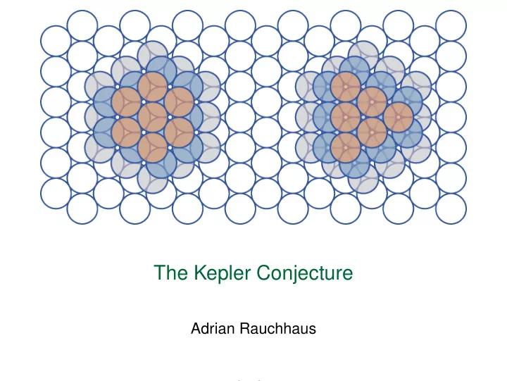
SLIDE 1 The Kepler Conjecture
Adrian Rauchhaus
SLIDE 2
The Theorem
There is no packing of equally sized spheres in the Euclidean three-space with a higher average density than that of the cubic close packing and the hexagonal close packing (of π/ √ 18).
SLIDE 3
The Theorem
There is no packing of equally sized spheres in the Euclidean three-space with a higher average density than that of the cubic close packing and the hexagonal close packing (of π/ √ 18).
SLIDE 4
History of the problem
SLIDE 5
History of the problem
◮ Formulated by Johannes Kepler ca. 1600
SLIDE 6
History of the problem
◮ Formulated by Johannes Kepler ca. 1600 ◮ Part of Hilberts 18th problem
SLIDE 7
History of the problem
◮ Formulated by Johannes Kepler ca. 1600 ◮ Part of Hilberts 18th problem ◮ Fejes Tóth suggests the use of computers for solving ca.
1950
SLIDE 8
History of the problem
◮ Formulated by Johannes Kepler ca. 1600 ◮ Part of Hilberts 18th problem ◮ Fejes Tóth suggests the use of computers for solving ca.
1950
◮ Proven by Thomas Hales and Samuel Ferguson in 1998
SLIDE 9
History of the problem
◮ Formulated by Johannes Kepler ca. 1600 ◮ Part of Hilberts 18th problem ◮ Fejes Tóth suggests the use of computers for solving ca.
1950
◮ Proven by Thomas Hales and Samuel Ferguson in 1998 ◮ Formalization of the proof in the FlysPecK project from
2003 to 2014
SLIDE 10
The proof assistants
For the formal proof of the Kepler Conjecture three proof assistants were used:
SLIDE 11
The proof assistants
For the formal proof of the Kepler Conjecture three proof assistants were used:
◮ HOL Light
SLIDE 12
The proof assistants
For the formal proof of the Kepler Conjecture three proof assistants were used:
◮ HOL Light ◮ Isabelle HOL
SLIDE 13
The proof assistants
For the formal proof of the Kepler Conjecture three proof assistants were used:
◮ HOL Light ◮ Isabelle HOL ◮ HOL Zero
SLIDE 14
Formalization
◮ The density of an infinite packing V is the limit of the
density in finite spherical containers as the radius of the containers grows to infinity.
SLIDE 15
Formalization
◮ The density of an infinite packing V is the limit of the
density in finite spherical containers as the radius of the containers grows to infinity.
◮ Density is scale invariant → Sufficient to consider unit balls
SLIDE 16
Formalization
◮ The density of an infinite packing V is the limit of the
density in finite spherical containers as the radius of the containers grows to infinity.
◮ Density is scale invariant → Sufficient to consider unit balls ◮ Packing can be identified with the centers of the spheres
SLIDE 17 Formalization
◮ The density of an infinite packing V is the limit of the
density in finite spherical containers as the radius of the containers grows to infinity.
◮ Density is scale invariant → Sufficient to consider unit balls ◮ Packing can be identified with the centers of the spheres ◮ Definition of a packing in HOL Light:
|− packing V <=> ( ! u v . u IN V / \ v IN V / \ d i s t (u , v ) < &2 ==> u = v )
SLIDE 18
Formalization
Mathematical formalization of the Kepler Conjecture:
SLIDE 19
Formalization
Mathematical formalization of the Kepler Conjecture: ∀ packings V ∃ c ∈ R : ∀r ≥ 1 : |V ∩ Br(0)| ≤ π ∗ r 3/ √ 18 + c ∗ r 2
SLIDE 20
Formalization
Mathematical formalization of the Kepler Conjecture: ∀ packings V ∃ c ∈ R : ∀r ≥ 1 : |V ∩ Br(0)| ≤ π ∗ r 3/ √ 18 + c ∗ r 2 Formalization in HOL Light:
SLIDE 21 Formalization
Mathematical formalization of the Kepler Conjecture: ∀ packings V ∃ c ∈ R : ∀r ≥ 1 : |V ∩ Br(0)| ≤ π ∗ r 3/ √ 18 + c ∗ r 2 Formalization in HOL Light:
|− the_kepler_conjecture <=> ( ! V. packing V ==> (? c . ! r . &1 <= r ==> &(CARD(V INTER b a l l ( vec 0 , r ) ) ) <= pi ∗ r pow 3 / sqrt (&18) + c ∗ r pow 2) )
SLIDE 22
Main parts of the proof
The proof consists mainly of three parts of calculations:
SLIDE 23
Main parts of the proof
The proof consists mainly of three parts of calculations:
◮ the_nonlinear_inequalities
SLIDE 24
Main parts of the proof
The proof consists mainly of three parts of calculations:
◮ the_nonlinear_inequalities:
A list of nearly a thousand nonlinear inequalities
SLIDE 25
Main parts of the proof
The proof consists mainly of three parts of calculations:
◮ the_nonlinear_inequalities:
A list of nearly a thousand nonlinear inequalities
◮ import_tame_classification
SLIDE 26
Main parts of the proof
The proof consists mainly of three parts of calculations:
◮ the_nonlinear_inequalities:
A list of nearly a thousand nonlinear inequalities
◮ import_tame_classification:
Possible counterexamples can be identified as tame (plane) graphs. Every tame graph is isomorphic to an element of a finite list of plane graphs.
SLIDE 27
Main parts of the proof
The proof consists mainly of three parts of calculations:
◮ the_nonlinear_inequalities:
A list of nearly a thousand nonlinear inequalities
◮ import_tame_classification:
Possible counterexamples can be identified as tame (plane) graphs. Every tame graph is isomorphic to an element of a finite list of plane graphs.
◮ linear_programming_results
SLIDE 28
Main parts of the proof
The proof consists mainly of three parts of calculations:
◮ the_nonlinear_inequalities:
A list of nearly a thousand nonlinear inequalities
◮ import_tame_classification:
Possible counterexamples can be identified as tame (plane) graphs. Every tame graph is isomorphic to an element of a finite list of plane graphs.
◮ linear_programming_results:
A large collection of linear programs that are infeasible for the possible counterexamples.
SLIDE 29
Main parts of the proof
The proof consists mainly of three parts of calculations:
◮ the_nonlinear_inequalities:
A list of nearly a thousand nonlinear inequalities
◮ import_tame_classification:
Possible counterexamples can be identified as tame (plane) graphs. Every tame graph is isomorphic to an element of a finite list of plane graphs.
◮ linear_programming_results:
A large collection of linear programs that are infeasible for the possible counterexamples. Since the proof was not obtained in a single session the following theorem was formalized:
SLIDE 30
Main parts of the proof
The proof consists mainly of three parts of calculations:
◮ the_nonlinear_inequalities:
A list of nearly a thousand nonlinear inequalities
◮ import_tame_classification:
Possible counterexamples can be identified as tame (plane) graphs. Every tame graph is isomorphic to an element of a finite list of plane graphs.
◮ linear_programming_results:
A large collection of linear programs that are infeasible for the possible counterexamples. Since the proof was not obtained in a single session the following theorem was formalized:
|- the_nonlinear_inequalities /\ import_tame_classification ==> the_kepler_conjecture
SLIDE 31
Idea of the proof
Transform the problem into a problem of distances between spheres:
SLIDE 32
Idea of the proof
Transform the problem into a problem of distances between spheres:
◮ Assume an arbitrary packing V
SLIDE 33
Idea of the proof
Transform the problem into a problem of distances between spheres:
◮ Assume an arbitrary packing V ◮ Divide the Euclidean space into Marchal cells
SLIDE 34
Idea of the proof
Transform the problem into a problem of distances between spheres:
◮ Assume an arbitrary packing V ◮ Divide the Euclidean space into Marchal cells:
Vertices of the cells are spheres on the boundary, edges are line segments between vertices along the boundary of the cell
SLIDE 35
Idea of the proof
Transform the problem into a problem of distances between spheres:
◮ Assume an arbitrary packing V ◮ Divide the Euclidean space into Marchal cells:
Vertices of the cells are spheres on the boundary, edges are line segments between vertices along the boundary of the cell
◮ Define some edges as critcal if they satisfy a specific
length condition
SLIDE 36
Idea of the proof
Transform the problem into a problem of distances between spheres:
◮ Assume an arbitrary packing V ◮ Divide the Euclidean space into Marchal cells:
Vertices of the cells are spheres on the boundary, edges are line segments between vertices along the boundary of the cell
◮ Define some edges as critcal if they satisfy a specific
length condition
◮ Cells that share critical edges form a cell cluster
SLIDE 37 Idea of the proof
Transform the problem into a problem of distances between spheres:
◮ Assume an arbitrary packing V ◮ Divide the Euclidean space into Marchal cells:
Vertices of the cells are spheres on the boundary, edges are line segments between vertices along the boundary of the cell
◮ Define some edges as critcal if they satisfy a specific
length condition
◮ Cells that share critical edges form a cell cluster ◮ Assign a real number Γ(ǫ, X) to the critical cells, depending
- n volume, angles between edges and lengths of edges
SLIDE 38 Idea of the proof
The Kepler conjecture can be represented as a local
- ptimization problem by using two inequalities:
SLIDE 39 Idea of the proof
The Kepler conjecture can be represented as a local
- ptimization problem by using two inequalities:
- 1. Cell-cluster inequality:
∀ critical edges ǫ :
Γ(ǫ, X) ≥ 0 X a cell, C the cell cluster
SLIDE 40 Idea of the proof
The Kepler conjecture can be represented as a local
- ptimization problem by using two inequalities:
- 1. Cell-cluster inequality:
∀ critical edges ǫ :
Γ(ǫ, X) ≥ 0 X a cell, C the cell cluster
- 2. Local annulus inequality:
SLIDE 41 Idea of the proof
The Kepler conjecture can be represented as a local
- ptimization problem by using two inequalities:
- 1. Cell-cluster inequality:
∀ critical edges ǫ :
Γ(ǫ, X) ≥ 0 X a cell, C the cell cluster
- 2. Local annulus inequality:
Constant ball annulus A = {x ∈ R3 : 2 ≤ x ≤ 2.52}
SLIDE 42 Idea of the proof
The Kepler conjecture can be represented as a local
- ptimization problem by using two inequalities:
- 1. Cell-cluster inequality:
∀ critical edges ǫ :
Γ(ǫ, X) ≥ 0 X a cell, C the cell cluster
- 2. Local annulus inequality:
Constant ball annulus A = {x ∈ R3 : 2 ≤ x ≤ 2.52} f(t) := 2.52−t
2.52−2
SLIDE 43 Idea of the proof
The Kepler conjecture can be represented as a local
- ptimization problem by using two inequalities:
- 1. Cell-cluster inequality:
∀ critical edges ǫ :
Γ(ǫ, X) ≥ 0 X a cell, C the cell cluster
- 2. Local annulus inequality:
Constant ball annulus A = {x ∈ R3 : 2 ≤ x ≤ 2.52} f(t) := 2.52−t
2.52−2
∀V ⊂ A :
f(v) ≤ 12
SLIDE 44
Figure: Constant ball annulus
SLIDE 45
Figure: Constant ball annulus
SLIDE 46
Intermediate result
◮ Cell-cluster inequality is proven by solving a few hundred
nonlinear inequalities
SLIDE 47
Intermediate result
◮ Cell-cluster inequality is proven by solving a few hundred
nonlinear inequalities
◮ Proving the local annulus inequality refutes all possible
counterexamples
SLIDE 48
Intermediate result
◮ Cell-cluster inequality is proven by solving a few hundred
nonlinear inequalities
◮ Proving the local annulus inequality refutes all possible
counterexamples This leads to the following intermediate result:
|− the_nonlinear_inequalities / \ ( ! V. c e l l _ c l u s t e r _ i n e q u a l i t y V) / \ ( ! V. packing V / \ V SUBSET ball_annulus ==> local_annulus_inequality V) ==> the_kepler_conjecture
SLIDE 49
Nonlinear inequalities
◮ Most of the inequalities have the form:
∀x, x ∈ D ⇒ f1(x) < 0 ∧ · · · ∧ fk(x) < 0 with n ∈ N, n ≤ 6, D = [a1, b1] × · · · × [an, bn] and x = (x1, . . . , xn)
SLIDE 50
Nonlinear inequalities
◮ Most of the inequalities have the form:
∀x, x ∈ D ⇒ f1(x) < 0 ∧ · · · ∧ fk(x) < 0 with n ∈ N, n ≤ 6, D = [a1, b1] × · · · × [an, bn] and x = (x1, . . . , xn)
◮ Basic arithmetic operations, square roots, trigonometric
functions and the analytic continuation of arctan(√x)/√x to the region x > −1
SLIDE 51
Nonlinear inequalities
The inequalities are solved by using interval arithmetics:
SLIDE 52
Nonlinear inequalities
The inequalities are solved by using interval arithmetics:
◮ Numbers are approximated by intervalls, e.g. π is
represented by [3.14, 3.15]
SLIDE 53
Nonlinear inequalities
The inequalities are solved by using interval arithmetics:
◮ Numbers are approximated by intervalls, e.g. π is
represented by [3.14, 3.15]
◮ Let f : R → R
SLIDE 54
Nonlinear inequalities
The inequalities are solved by using interval arithmetics:
◮ Numbers are approximated by intervalls, e.g. π is
represented by [3.14, 3.15]
◮ Let f : R → R
Then the interval extension F : IR → IR satisfies ∀I ∈ IR, {f(x) : x ∈ I} ⊂ F(I)
SLIDE 55
Nonlinear inequalities
The inequalities are solved by using interval arithmetics:
◮ Numbers are approximated by intervalls, e.g. π is
represented by [3.14, 3.15]
◮ Let f : R → R
Then the interval extension F : IR → IR satisfies ∀I ∈ IR, {f(x) : x ∈ I} ⊂ F(I)
◮ Sum of intervals:
[a1, b1] ⊕ [a2, b2] = [a, b] for some a ≤ a1 + a2 and b ≥ b1 + b2
SLIDE 56
Nonlinear inequalities
The inequalities are solved by using interval arithmetics:
◮ Numbers are approximated by intervalls, e.g. π is
represented by [3.14, 3.15]
◮ Let f : R → R
Then the interval extension F : IR → IR satisfies ∀I ∈ IR, {f(x) : x ∈ I} ⊂ F(I)
◮ Sum of intervals:
[a1, b1] ⊕ [a2, b2] = [a, b] for some a ≤ a1 + a2 and b ≥ b1 + b2
◮ Other arithmetic operations defined analogously
SLIDE 57
Nonlinear inequalities
Problem:
◮ Natural interval extensions often imprecise
SLIDE 58
Nonlinear inequalities
Problem:
◮ Natural interval extensions often imprecise
Solution:
◮ Divide intervals into subintervals
SLIDE 59
Nonlinear inequalities
Problem:
◮ Natural interval extensions often imprecise
Solution:
◮ Divide intervals into subintervals ◮ Use interval extensions based on Taylor approximations
SLIDE 60
Nonlinear inequalities
Problem:
◮ Natural interval extensions often imprecise
Solution:
◮ Divide intervals into subintervals ◮ Use interval extensions based on Taylor approximations
Through partitioning of domains one obtains more than 23000 nonlinear inequalities.
SLIDE 61
Nonlinear inequalities
Problem:
◮ Natural interval extensions often imprecise
Solution:
◮ Divide intervals into subintervals ◮ Use interval extensions based on Taylor approximations
Through partitioning of domains one obtains more than 23000 nonlinear inequalities. These can be verified in about 5000 hours in HOL Light.
SLIDE 62
Tame classification
Plane graphs:
SLIDE 63
Tame classification
Plane graphs:
◮ n-tuples of data including a list of faces
SLIDE 64
Tame classification
Plane graphs:
◮ n-tuples of data including a list of faces ◮ tame, if faces are triangles or hexagonal and the
admissible weight is bounded
SLIDE 65
Tame classification
Plane graphs:
◮ n-tuples of data including a list of faces ◮ tame, if faces are triangles or hexagonal and the
admissible weight is bounded
◮ Tame graphs collected in a text file called archive
SLIDE 66
Tame classification
Plane graphs:
◮ n-tuples of data including a list of faces ◮ tame, if faces are triangles or hexagonal and the
admissible weight is bounded
◮ Tame graphs collected in a text file called archive ◮ Possible counterexamples encoded as tame graphs
SLIDE 67
Tame classification
Goal: ⊢”g ∈ PlaneGraphs” and ”tame g” implies ”fgraph g ∈≃ Archive” fgraph maps graph to the list of faces
SLIDE 68
Tame classification
Goal: ⊢”g ∈ PlaneGraphs” and ”tame g” implies ”fgraph g ∈≃ Archive” fgraph maps graph to the list of faces In HOL Light:
|− import_tame_classifiation <==> ( ! g . g IN PlaneGraphs / \ tame g ==> fgraph g IN_simeq archive )
SLIDE 69
Tame classification
Enumeration of the tame graphs:
SLIDE 70
Tame classification
Enumeration of the tame graphs:
◮ Start with a polygon as a seed graph
SLIDE 71
Tame classification
Enumeration of the tame graphs:
◮ Start with a polygon as a seed graph ◮ Obtain new graphs by dividing the faces of the graph
SLIDE 72
Tame classification
Enumeration of the tame graphs:
◮ Start with a polygon as a seed graph ◮ Obtain new graphs by dividing the faces of the graph ◮ The function next_tame maps graph to obtainable tame
graphs
SLIDE 73
Tame classification
Enumeration of the tame graphs:
◮ Start with a polygon as a seed graph ◮ Obtain new graphs by dividing the faces of the graph ◮ The function next_tame maps graph to obtainable tame
graphs
◮ next_tame produces the set TameEnum
SLIDE 74
Tame classification
Enumeration of the tame graphs:
◮ Start with a polygon as a seed graph ◮ Obtain new graphs by dividing the faces of the graph ◮ The function next_tame maps graph to obtainable tame
graphs
◮ next_tame produces the set TameEnum
Isabelle can automatically compute: ⊢ fgraph ’ TameEnum ⊆≃ Archive
SLIDE 75
Tame enumeration
At this point we know:
◮ An infinite possible counterexample can be reduced to a
finite packing
◮ Finite packings can be encoded as plane graphs ◮ Only finitely many tame plane graphs exist
SLIDE 76
Linear programs
◮ Counterexamples have to fulfill a list of inequalities
SLIDE 77
Linear programs
◮ Counterexamples have to fulfill a list of inequalities ◮ Substitution leads to linear relaxations
SLIDE 78
Linear programs
◮ Counterexamples have to fulfill a list of inequalities ◮ Substitution leads to linear relaxations
Example: x + x2 ≤ 3 and x ≥ 2
SLIDE 79
Linear programs
◮ Counterexamples have to fulfill a list of inequalities ◮ Substitution leads to linear relaxations
Example: x + x2 ≤ 3 and x ≥ 2 Substitute y := x2
SLIDE 80
Linear programs
◮ Counterexamples have to fulfill a list of inequalities ◮ Substitution leads to linear relaxations
Example: x + x2 ≤ 3 and x ≥ 2 Substitute y := x2 This implies x + y ≤ 3 and y ≥ 4
SLIDE 81
Linear programs
◮ Counterexamples have to fulfill a list of inequalities ◮ Substitution leads to linear relaxations
Example: x + x2 ≤ 3 and x ≥ 2 Substitute y := x2 This implies x + y ≤ 3 and y ≥ 4 Adding x ≥ 2 and y ≥ 4 leads to x + y ≥ 6, a contradiction
SLIDE 82
Linear programs
◮ Counterexamples have to fulfill a list of inequalities ◮ Substitution leads to linear relaxations
Example: x + x2 ≤ 3 and x ≥ 2 Substitute y := x2 This implies x + y ≤ 3 and y ≥ 4 Adding x ≥ 2 and y ≥ 4 leads to x + y ≥ 6, a contradiction
◮ HOL Light solves equations over rational inequalities,
modifies them to integer inequalities
SLIDE 83
Linear programs
◮ Counterexamples have to fulfill a list of inequalities ◮ Substitution leads to linear relaxations
Example: x + x2 ≤ 3 and x ≥ 2 Substitute y := x2 This implies x + y ≤ 3 and y ≥ 4 Adding x ≥ 2 and y ≥ 4 leads to x + y ≥ 6, a contradiction
◮ HOL Light solves equations over rational inequalities,
modifies them to integer inequalities Example: x ≥ π
SLIDE 84
Linear programs
◮ Counterexamples have to fulfill a list of inequalities ◮ Substitution leads to linear relaxations
Example: x + x2 ≤ 3 and x ≥ 2 Substitute y := x2 This implies x + y ≤ 3 and y ≥ 4 Adding x ≥ 2 and y ≥ 4 leads to x + y ≥ 6, a contradiction
◮ HOL Light solves equations over rational inequalities,
modifies them to integer inequalities Example: x ≥ π ⇒ x ≥ 3, 14
SLIDE 85
Linear programs
◮ Counterexamples have to fulfill a list of inequalities ◮ Substitution leads to linear relaxations
Example: x + x2 ≤ 3 and x ≥ 2 Substitute y := x2 This implies x + y ≤ 3 and y ≥ 4 Adding x ≥ 2 and y ≥ 4 leads to x + y ≥ 6, a contradiction
◮ HOL Light solves equations over rational inequalities,
modifies them to integer inequalities Example: x ≥ π ⇒ x ≥ 3, 14 ⇔ 100x ≥ 314
SLIDE 86
Linear programs
◮ Counterexamples have to fulfill a list of inequalities ◮ Substitution leads to linear relaxations
Example: x + x2 ≤ 3 and x ≥ 2 Substitute y := x2 This implies x + y ≤ 3 and y ≥ 4 Adding x ≥ 2 and y ≥ 4 leads to x + y ≥ 6, a contradiction
◮ HOL Light solves equations over rational inequalities,
modifies them to integer inequalities Example: x ≥ π ⇒ x ≥ 3, 14 ⇔ 100x ≥ 314
◮ Inaccurate approximations lead to case distinctions
SLIDE 87
Linear programs
◮ Counterexamples have to fulfill a list of inequalities ◮ Substitution leads to linear relaxations
Example: x + x2 ≤ 3 and x ≥ 2 Substitute y := x2 This implies x + y ≤ 3 and y ≥ 4 Adding x ≥ 2 and y ≥ 4 leads to x + y ≥ 6, a contradiction
◮ HOL Light solves equations over rational inequalities,
modifies them to integer inequalities Example: x ≥ π ⇒ x ≥ 3, 14 ⇔ 100x ≥ 314
◮ Inaccurate approximations lead to case distinctions ◮ In total 43078 linear programs
SLIDE 88
Linear programs
◮ Counterexamples have to fulfill a list of inequalities ◮ Substitution leads to linear relaxations
Example: x + x2 ≤ 3 and x ≥ 2 Substitute y := x2 This implies x + y ≤ 3 and y ≥ 4 Adding x ≥ 2 and y ≥ 4 leads to x + y ≥ 6, a contradiction
◮ HOL Light solves equations over rational inequalities,
modifies them to integer inequalities Example: x ≥ π ⇒ x ≥ 3, 14 ⇔ 100x ≥ 314
◮ Inaccurate approximations lead to case distinctions ◮ In total 43078 linear programs ◮ Solvable in about 15 hours
SLIDE 89
Linear programs
◮ Counterexamples have to fulfill a list of inequalities ◮ Substitution leads to linear relaxations
Example: x + x2 ≤ 3 and x ≥ 2 Substitute y := x2 This implies x + y ≤ 3 and y ≥ 4 Adding x ≥ 2 and y ≥ 4 leads to x + y ≥ 6, a contradiction
◮ HOL Light solves equations over rational inequalities,
modifies them to integer inequalities Example: x ≥ π ⇒ x ≥ 3, 14 ⇔ 100x ≥ 314
◮ Inaccurate approximations lead to case distinctions ◮ In total 43078 linear programs ◮ Solvable in about 15 hours ◮ This concludes the proof
SLIDE 90
References
◮ Hales, T., Adams, M., Bauer, G., Dang, T., Harrison, J.,
Hoang, L., . . . Zumkeller, R. (2017). A formal proof of the Kepler Conjecture. Forum of Mathematics, Pi, 5, E2. doi:10.1017/fmp.2017.1
◮ Hales, T. C., Dense Sphere Packings: a Blueprint for
Formal Proofs, London Mathematical Society Lecture Note Series, 400 (Cambridge University Press, 2012)
◮ George G. Szpiro. Die Keplersche Vermutung.
Springer-Verlag, 2011 Pictures:
◮ https://hexnet.org/content/close-packing-spheres ◮ https://upload.wikimedia.org/wikipedia/commons/2/2e/
Closepacking.svg