The k -mer index k -mer index 5 0 CC Earlier in this course, we - - PDF document

Bioinformatics Algorithms

(Fundamental Algorithms, module 2)

Zsuzsanna Lipt´ ak

Masters in Medical Bioinformatics academic year 2018/19, II. semester

Suffix Trees (and other string indexes)1

1Some of these slides are based on slides of Jens Stoye’s.

Text indexes

Let T be a string of length n over alphabet Σ (which we refer to as text in the following). A text index (or string index) is a data structure built on the text which allows to answer a certain type of query (e.g. pattern matching) without traversing the whole text. Typically, we want

• 1. the index not to use too much space (linear or sublinear in n), and
• 2. the query time to be fast (ideally: independent of n).

2 / 17

A common string problem: Pattern matching

Pattern matching (aka exact string matching) is at the core of almost every text-managing application.

Pattern matching

Given a (typically long) string T (the text), and a (typically much shorter) string P (the pattern) over the same alphabet Σ, find all occurrences of P as substring of T.

Variants:

• output all occurrences of P in T — ”all-occurrences version”
• decide whether P occurs in T (yes - no) — ”decision version”
• output the number of occurrences of P in T — ”counting version”

We usually refer to the number of occurrences of P as occP.

3 / 17

Pattern matching

Pattern matching (p.m.)

text: T = T1 . . . Tn of length n, pattern: P = P1 . . . Pm of length m

• The best non-index-based algorithms solve this problem in time

O(n + m) (e.g. Knuth-Morris-Pratt)

• This is optimal, since one has to read both strings at least once.
• But not tolerable with the data sizes we are seeing now!
• That is why we need text indexes.

4 / 17

The k-mer index

5 / 17

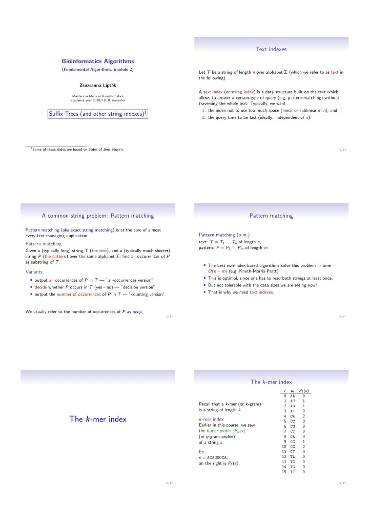
The k-mer index

Recall that a k-mer (or k-gram) is a string of length k.

k-mer index

Earlier in this course, we saw the k-mer profile, Pk(s) (or q-gram profile)

• f a string s.

Ex.

s = ACAGGGCA,

• n the right is P2(s).

r ur P2(s) AA 1 AC 1 2 AG 1 3 AT 4 CA 2 5 CC 6 CG 7 CT 8 GA 9 GC 1 10 GG 2 11 GT 12 TA 13 TC 14 TG 15 TT

6 / 17

The k-mer index

Replacing the number of occurrences by the occurrences themselves, we get the k-mer index of s.

Ex.

s = ACAGGGCA,

• n the right 2-mer index of s.

Analysis (for p.m.)

Space: total space is O(σk + n), since no. of rows = σk and total number of entries = n k + 1. Time (p.m.): O(k) for decision, O(k + occP) for all-occurrences.

r ur k-mer index of s AA 1 AC 1 2 AG 3 3 AT 4 CA 2, 7 5 CC 6 CG 7 CT 8 GA 9 GC 6 10 GG 4, 5 11 GT 12 TA 13 TC 14 TG 15 TT

7 / 17

The k-mer index

Replacing the number of occurrences by the occurrences themselves, we get the k-mer index of s.

Ex.

s = ACAGGGCA,

• n the right 2-mer index of s.

Analysis (for p.m.)

Space: total space is O(σk + n), since no. of rows = σk and total number of entries = n k + 1. Time (p.m.): O(k) for decision, O(k + occP) for all-occurrences. N.B.: works only for patterns of length exactly k

r ur k-mer index of s AA 1 AC 1 2 AG 3 3 AT 4 CA 2, 7 5 CC 6 CG 7 CT 8 GA 9 GC 6 10 GG 4, 5 11 GT 12 TA 13 TC 14 TG 15 TT

7 / 17

The suffix tree

8 / 17

The suffix tree

T = BANANA$ (add sentinel character $ / 2 Σ)

labels only conceptual!

A NA BANANA$ NA$ $ $ $ N A $ NA$

7 6 4 2 1 5 3

two pointers into string

[2,2] [3,4] [1,7] [5,7] [7,7] [7,7] [7,7] [ 3 , 4 ] [7,7] [5,7]

7 6 4 2 1 5 3 9 / 17

The suffix tree

Given T string over Σ (finite ordered alphabet), and $ 62 Σ.

Definitions

• ST(T) is a rooted tree with edge-labels from (Σ [ {$})+ such that
• the labels of all edges outgoing from a node begin with different

characters;

• the paths from the root to the leaves of ST(T) spell the suffixes of T$;
• each node in ST(T) is either the root, a leaf, or a branching node;
• L(u) is the path-label of node u: the concatenation of edge labels on

the path from the root to u,

• a leaf v has leaf-label i if and only if L(v) = Ti . . . Tn$ (i’th suffix),
• sd(v) is the string-depth of a node v is the length of its path-label,
• a locus (u, d) is a position on an edge (v, u) where u is a node of

ST(T) and sd(v) < d  sd(u): d is the string-depth of locus (u, d).

10 / 17

• N.B.: the edge labels are not stored explicitly:
• they are represented by two pointers [b, e] into T: beginning and end
• f an occurrence of the edge label;
• this representation is not necessarily unique
• e.g. in the example, any edge with label NA can be represented by

[3, 4] or [5, 6]

labels only conceptual!

A NA B A N A N A $ NA$ $ $ $ N A $ NA$

7 6 4 2 1 5 3

two pointers into string

[2,2] [3,4] [ 1 , 7 ] [5,7] [7,7] [7,7] [7,7] [ 3 , 4 ] [7,7] [5,7]

7 6 4 2 1 5 3 11 / 17

Suffix tree properties

• The leaves of ST(T) correspond to the suffixes of T$.
• ST(T) represents exactly the substrings of T$: there is a one-to-one

correspondence between loci in ST(T) (possibly within an edge) and substrings of T$.

• This allows us to define locus(P) for a substring P of T.
• The leaves in the subtree under a locus(P) correspond to the

(beginning positions of) P’s occurrences in T$: one-to-one correspondence between leaves in subtree under locus(P) and

• ccurrences of substring P.
• ST(T) requires O(n) space (details next).

MAGIC!

The suffix tree represents a possibly quadratic number of objects (the substrings) in linear space!

12 / 17

Space usage of suffix trees

Lemma:

ST(T) requires O(n) space.

Proof sketch:

• 1. ST(T) has exactly n + 1 leaves (one for each suffix).
• 2. Each internal node is branching, therefore there are at most n internal

nodes.

• 3. A tree with at most 2n + 1 nodes has at most 2n edges.
• 4. Each node can be represented in constant space.
• 5. Each edge is labeled by a substring of T$ and hence can be

represented by a pair of pointers [i, j] into T$.

13 / 17

The suffix array

14 / 17

The suffix array

Definition

The SA is a permutation of {1, 2, . . . , n + 1} s.t. SA[i] = j if the j’th suffix Sufj = Tj · · · Tn$ is the i’th among all suffixes in lexicographic order. Example: T = BANANA$ SA = [

1

7,

2

6,

3

4,

4

2,

5

1,

6

5,

7

3]

i SA Sufi 1 7 $ 2 6 A$ 3 4 ANA$ 4 2 ANANA$ 5 1 BANANA$ 6 5 NA$ 7 3 NANA$ Note $ is smaller than all other characters.

15 / 17

The suffix array

Suffix tree

A NA BANANA$ NA$ $ $ $ NA $ NA$

7 6 4 2 1 5 3

(Note that children of inner nodes are

• rdered acc. to the alphabet’s order.)

Suffix array

SA = [7,6,4,2,1,5,3]

N.B.

When reading the leaves of the ST from left-to-right, we get the SA. One can imagine the suffix array as the leaves of the suffix tree that fell down and stayed in order . . .

16 / 17

Some Applications of Suffix Trees/Suffix Arrays

• exact string matching
• exact set matching
• text statistics
• DNA contamination problem
• common substrings of more than two strings
• matching statistics
• overlap computation (all-pairs prefix-suffix matching)
• exact repeats and palindromes problem
• tandem repeats problem
• shortest unique substring
• maximal unique matches
• approximate string matching (k-mismatch and k-differences)
• computation of the q-gram distance
• Lempel-Ziv data compression

17 / 17