The ideal free strategy with weak Allee effect Daniel S. Munther - - PowerPoint PPT Presentation

The ideal free strategy with weak Allee effect

Daniel S. Munther

York University

April 12, 2013

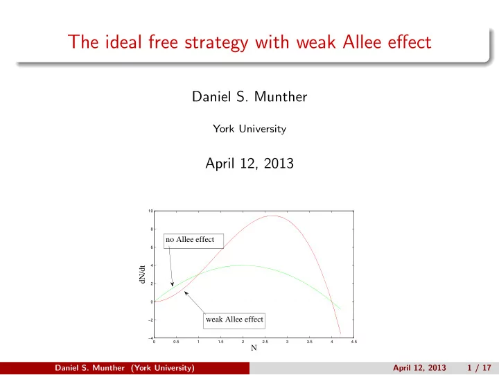
0.5 1 1.5 2 2.5 3 3.5 4 4.5 −4 −2 2 4 6 8 10

N dN/dt no Allee effect weak Allee effect Daniel S. Munther (York University) April 12, 2013 1 / 17

1 Introduction 2 Ideal Free Distribution 3 Adding Allee effects 4 Conclusions

Daniel S. Munther (York University) April 12, 2013 2 / 17

Introduction

Ecology and dispersal

Which patterns of dispersal provide an evolutionary advantage in a variable environment? Unbiased dispersal - independent of habitat, population density, etc. Biased dispersal - depends on one or more factors

Daniel S. Munther (York University) April 12, 2013 3 / 17

Introduction

Generalized two species model

(Cantrell et al. 2010) ut = µ∇ · [∇u − u∇P(x)] + u[m(x) − u − v] in Ω × (0, ∞), vt = ν∇ · [∇v − v∇Q(x)] + v[m(x) − u − v] in Ω × (0, ∞), (1) [∇u − u∇P] · n = [∇v − v∇Q] · n = 0 on ∂Ω × (0, ∞) Species have same population dynamics but different movement strategies m(x) > 0 is nonconstant (spatially inhomogeneous) Semi-trivial steady states: (u∗, 0) and (0, v∗) Is there a strategy P(x) which cannot be invaded?

Daniel S. Munther (York University) April 12, 2013 4 / 17

Ideal Free Distribution

Single species distribution

Diffusion creates a mismatch between population density at steady state and habitat quality m(x) (Cantrell et al. 2010) µ∇ · [∇u − u∇P(x)] + u[m(x) − u] = 0 in Ω, [∇u − u∇P(x)] · n = 0

• n

∂Ω. If P(x) = ln m(x), u ≡ m is a positive steady state. No net movement: ∇u − u∇P(x) = ∇m − m∇ ln m = ∇m − ∇m = 0 Fitness equilibrated throughout the habitat: m

u ≡ 1.

We call P = ln m an Ideal Free Strategy (IFS).

Daniel S. Munther (York University) April 12, 2013 5 / 17

Ideal Free Distribution

Habitat Selection Theory (Fretwell and Lucas 1970):

1 Choose most suitable habitat (ideal) 2 Can move into any desired region (free)

Ideal Free Distribution: A species will aggregate in a location proportionately to the amount of available resources in that location

Daniel S. Munther (York University) April 12, 2013 6 / 17

Ideal Free Distribution

Evolutionary stable strategy

Cantrell et al. showed that P = ln m is a local evolutionary stable strategy (ESS) and no other strategy can be a local ESS. Theorem (Averill et al.) Suppose that P = ln m and Q − ln m is nonconstant. Then (0, v∗) is unstable and (u∗, 0) is globally asymptotically stable. Biologically, P = ln m is a global ESS. Main Question: Does this result still hold when u(m − u − v) is replaced by u2(m − u − v) in model (1)?

Daniel S. Munther (York University) April 12, 2013 7 / 17

Adding Allee effects

Modified model (Munther, JDE 2013)

ut = µ∇ · [∇u − u∇ ln(m)] + u2(m − u − v) in Ω × (0, ∞), vt = ν∇ · [∇v − βv∇ ln(m)] + v(m − u − v) in Ω × (0, ∞), (2) [∇u − u∇ ln(m)] · n = [∇v − βv∇ ln(m)] · n = 0

• n

∂Ω × (0, ∞). Why is this interesting? u is subject to weak Allee effect (species no longer have the same population dynamics) Interplay between IFS and weak Allee effect Invasion dynamics not useful for any β ∈ [0, ∞)

Daniel S. Munther (York University) April 12, 2013 8 / 17

Adding Allee effects

β = 0 case

Theorem (1) Suppose m ∈ C 2(¯ Ω) is positive and non-constant. Then for β = 0 and any µ, ν > 0, any solution (u, v) of (2) with nonnegative, not identically zero initial data converges to (m, 0) in L∞(Ω) as t → ∞. u cannot only invade v, but it drives v to extinction no matter its diffusion rate IFS offsets the weak Allee effect

Daniel S. Munther (York University) April 12, 2013 9 / 17

Adding Allee effects

Proof of Theorem (1)

Recast model as dynamical system S[u, v] on C(¯ Ω) × C(¯ Ω). The order interval G = [(0, v∗), (m, 0)] is a basin of attraction. Define E(u, v) =

• Ω

m2 u + 2m ln u − u + v2 2 . dE dt = −µ

• Ω

2m|∇(u/m)|2(1−(u/m)) (u/m)3

− ν

• Ω |∇v|2

−

• Ω((m − u)2 − v2)(m − u − v) ≤ 0 on G.

By LaSalle’s invariance principal for infinite dimensions, S[u, v] → (m, 0).

Daniel S. Munther (York University) April 12, 2013 10 / 17

Adding Allee effects

β ≪ 1 case

Theorem (2) Suppose m ∈ C 2(¯ Ω) is positive and non-constant. Then there exists 0 < β∗ < 1 such that for all β ∈ (0, β∗) and any µ, ν > 0, any solution (u, v) of (2) with nonnegative, not identically zero initial data converges to (m, 0) in L∞(Ω) as t → ∞. Again, u is sole winner as IFS is able to still offset the Allee effect. Proof for Theorem (2) is more tricky.

Daniel S. Munther (York University) April 12, 2013 11 / 17

Adding Allee effects

Remarks

Conjecture: Theorem (2) holds for all β ∈ (0, 1). First, (0, v∗) is unstable for β ∈ (0, 1), since

• Ω m2(m − v∗) > 0.

Second, numerics indicate no positive steady states. For the β = 1 case, both species are playing IFS and hence coexist. System (2) has a continuum of positive steady states of the form (sm, (1 − s)m) for s ∈ (0, 1). For the β >> 1 case, we can show (0, v∗) is unstable. Conjecture: u (IFS) should be the sole winner as in Theorem (2). For m with single max in Ω, we can prove this (Adrian Lam).

Daniel S. Munther (York University) April 12, 2013 12 / 17

Adding Allee effects

Intermediate β ∈ (1, 1 + ǫ) case

Current work (with Adrian Lam): We can show that

• Ω m2(m − v∗) < 0.

Using upper/lower solution argument, eliminate positive steady states near (0, v∗). By monotonicity, we can show that (0, v∗) is locally asymptotically stable. Fundamentally different: The winning strategy is no longer a “resource matching” strategy. Biological explanation?

Daniel S. Munther (York University) April 12, 2013 13 / 17

Adding Allee effects

Intermediate β > 1 case

Numerical example:

0.1 0.2 0.3 0.4 0.5 0.6 0.7 0.8 0.9 1 0.5 1 1.5 2 2.5 3 3.5 T=1.5 Distance x Density u v m 0.1 0.2 0.3 0.4 0.5 0.6 0.7 0.8 0.9 1 0.5 1 1.5 2 2.5 3 3.5 4 T=105 Distance x Density u v m

Figure: m(x) = 3e−50(x−.2)2 + 1.7e−40(x−.8)2 + .2 (black) and u (red) and v (blue), µ = 1000, ν = 1000, β = 1.7 a) two species at T = 1.5, b) T = 105. The growth rate for u near x = 0.8 is m(x) − v(x, t) > 0 for all t > T0. For β in this range, v can defeat u even when u has significant initial numbers.

Daniel S. Munther (York University) April 12, 2013 14 / 17

Conclusions

Summary: For β ∈ [0, 1) and [β∗, ∞), the ideal free disperser dominates. For β = 1, coexistence as both species are ideal free dispersers For intermediate β > 1, the ideal free strategy cannot invade. Future work: Prove global stability of (0, v∗) for β ∈ (1, 1 + ǫ). u subject to a strong Allee effect

Daniel S. Munther (York University) April 12, 2013 15 / 17

Conclusions

References

R.S. Cantrell, C. Cosner, and Y. Lou, Evolution of dispersal and ideal free distribution, Math Bios. Eng., Vol 7 (2010) 17-36.

• I. Averill, Y. Lou, and D. Munther, On several conjectures from

evolution of dispersal, J. Biol. Dynamics, 6 (2012) 117-130.

• D. Munther, The ideal free strategy with weak Allee effect, J.

Differential Equations, 254 (2013) 1728-1740.

Daniel S. Munther (York University) April 12, 2013 16 / 17

Conclusions

Acknowledgement

Adrian Lam (MBI), Yuan Lou (OSU), and Jianhong Wu Support: NSERC Canada Research Chairs Program Fields Institute Mitacs and Mprime Centre for Disease Modeling

Daniel S. Munther (York University) April 12, 2013 17 / 17