The GENESIS of QUANTUM MECHANICS The quantum theory had its - PowerPoint PPT Presentation

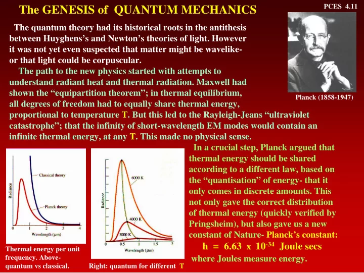
PCES 4.11 The GENESIS of QUANTUM MECHANICS The quantum theory had its historical roots in the antithesis between Huyghens’s and Newton’s theories of light. However it was not yet even suspected that matter might be wavelike- or that light could be corpuscular. The path to the new physics started with attempts to understand radiant heat and thermal radiation. Maxwell had shown the “equipartition theorem”; in thermal equilibrium, Planck (1858-1947) all degrees of freedom had to equally share thermal energy, proportional to temperature T. But this led to the Rayleigh-Jeans “ultraviolet catastrophe”; that the infinity of short-wavelength EM modes would contain an infinite thermal energy, at any T. This made no physical sense. In a crucial step, Planck argued that thermal energy should be shared according to a different law, based on the “quantisation” of energy- that it only comes in discrete amounts. This not only gave the correct distribution of thermal energy (quickly verified by Pringsheim), but also gave us a new constant of Nature- Planck’s constant: h = 6.63 x 10 -34 Joule secs Thermal energy per unit frequency. Above- where Joules measure energy. quantum vs classical. Right: quantum for different T

PCES 4.12 ATOMS & ELECTRONS Dalton, in 1802, showed how to understand chemical combinations, if some elementary chemicals came in atomic units. Despite the evidence for atoms, and elements (classified by Mendeleev in the periodic table), their existence was still doubted in 1900. It was finally established by theoretical work of Dalton (1766-1844) Boltzmann (1844-1906) Maxwell, Boltzmann & Einstein- they showed how one could quantitatively understand gas dynamics, as well as the random “Brownian” motion of small particles in liquids, in terms of atomic motion and collisions. Atomic sizes were found to be ~ 1 A = 10 -10 m . Electrons were discovered by JJ Thompson in 1895 in gas discharges- their mass is 9.11 x 10 -31 kg . Einstein went much farther. He explained the “photoelectric effect” (the emission of electrons by a metal when light is shone on it), using Planck’s quantum hypothesis. He argued that light came in packets (“photons”) of energy E = h ν where ν is the frequency of the light. This explained why the electronic energy depended only on the light frequency, & not its intensity. Apparatus for observation of the Photoelectric effect- the photoelectric effect. threshold V is invariant.

PCES 4.13 ATOMIC SPECTRA It was confidently claimed by the French positivist philosopher A. Comte that nobody could ever know what the stars were made of. However the discovery that the “Fraunhofer lines” in the spectra of stars including the sun were the same as those in the spectra of elements on earth allowed a chemical analysis of the stars (reinforced when unknown lines in the solar spectrum were identified by Lockyer in 1868 to be from a newly- discovered element- he called it He. The question was- what was causing these lines? Above: emission and absorption spectra of H Right: spectra of stars (from Flammarion, 1880)

PCES 4.14 RADIOACTIVITY A development which seemed to be completely unrelated began with the discovery of radioactivity by H. Becquerel in 1896, and the demonstration by P. and M. Curie, in a series of painstaking experiments, that radioactivity was the transmutation of certain elements to others with the concomitant emission of high-energy invisible rays. Above: the shed in the Ecole Normale where they worked The isolation of new radioactive elements, and the mystery of the underlying physics, caused a sensation- particularly as the conservative French establishment refused to properly acknowledge the role of Marie Curie. By the time she was awarded her 2 nd Nobel prize (in the middle of a scandalous love affair with Langevin), she was famous around the world- and had to hide in England for 6 months from the French press. Pierre (1859-1906) and Marie Curie (1867-1934)

PCES 4.15 Discovery of the ATOMIC NUCLEUS The mystery of the radioactive elements was solved in brilliant work by Rutherford, mostly done with Soddy in McGill in 1904-07, between periods in Rutherford (1871-1937) Cambridge and Manchester. He tried to probe the distribution of charge inside the atom by firing fast radioactive particles at a very thin sheet of Gold leaf (only about 100,000 atoms thick). To his astonishment almost all the particles went straight through- except for a few that were very strongly scattered (see left). Unlike most experimentalists then (and now), Rutherford did not labour under the delusion that experimentalists should leave the thinking to the theorists. He promptly worked out a model theory which explained the results quantitatively- the positively charged particles were being repelled by a positively charged atomic nucleus, as shown at right. The nucleus was fantastically small- roughly 100,000 times smaller than the atom, or 10 -15 m across.

PCES 4.16 The BOHR ATOM The “old quantum theory” of Bohr gave a partial understanding of the Hydrogen spectrum. Bohr supposed a set of “allowed” orbits of electrons around a H nucleus, labeled by a “quantum number” n . N. Bohr (1885-1962) An atom could emit or absorb radiation in this theory only in discrete amounts- in “quantum jumps” between allowed orbits (shown at left for H). The energy of the radiation is E nm = h ν nm / 2 π = ( ε n - ε m ) where ν nm is the frequency of the radiation, and ε n & ε m are the allowed energies of the electrons. This gave an explanation of spectral lines- although there was no explanation of why the electron orbits had to be “quantized”.

PCES 4.17 MATTER WAVES To take the crucial next step it helped to not know too much. Prince Louis de Broglie, studying for his PhD in Paris, advanced the idea that matter was associated with waves, and the momentum p of the waves was given by p = h/ λ where λ is the wavelength of the matter wave. Because L. De Broglie Planck’s contant is so small, the wave effects (1892-1987) are undetectable except for very light systems. Suppose, eg., we have a mass 1 kg, moving at speed 1 m/s., so it has unit momentum (remember p = mv in classical physics). Then, since λ = h/p, we find the very small Atomic wave-functions Only the blue closes on wavelength of 6.63 x 10 -34 m. This is > 10 19 times smaller itself. than the atomic nucleus! However an electron moving at the same 1 m/s will have a wavelength λ = 6.63 x 10 -34 / 9.1 x 10 -31 m, just under a millimetre. Thus we should see wave interference and diffraction effects with electrons. These were found a few years after de Broglie’s prediction, by Davisson & Germer in the USA, and Thompson in Cambridge (see right). The quantization of momentum also gave a simple explanation of Bohr’s quantization rules for atomic orbits (see above); only orbits which could fit a wave in, and thus having definite Electron diffraction by wavelengths, were allowed . a small hole (Thompson)

PCES 4.18 The DISCOVERY of QUANTUM MECHANICS The great theoretical denouement came in 1925. I do not give the details of the theory here, but just sketch the historical development. This began with the “matrix mechanics” of Heisenberg, who found a mathematical way of relating results of W Heisenberg (1901-76) measurements on momentum & position- E Schrodinger (1887-1961) which gave the ‘Uncertainty principle’. His scheme was based on mathematics then unfamiliar to most. Soon after Schrodinger also gave what seemed a quite different theory, based on a “wave equation” for a matter wave. He was led to this via a deep analysis of the mathematics underlying particle and wave motion, extending old work of WR Hamilton. Although also difficult, this was more familiar territory for most physicists. Then, in what was a real surprise, Schrodinger showed the 2 theories were equivalent. Schrodinger’s equation showed how to find the “wave function” ψ (r,t) as a function of position r and time t for any given potential energy. An example is shown (left); a particle is confined to a box, and we see the allowed states, whose Wave-functions in a energy increases as their wavelength gets shorter. box, & energy levels

PCES 4.19 The PROBABILITY INTERPRETATION The question remained, after the quantum theory was complete- what was the connection between the quantum amplitudes and the physical world? The answer given by M Born was very startling, and changed physics M Born (1882-1970) irrevocably. He argued that the wave amplitudes could be Energy levels used only to describe the & wave-fns in Probability densities hard-walled PROBABILITY that some for same potential. box potential phenomenon would occur. The orange band is a Formally, the probability position resolution. that we see a system at, say, a position r, is given by P(r) = | ψ (r)| 2 which means that we take the MAGNITUDE of the wave-function, & square it, to get the probability. Oscillator probability density Oscillator energy levels