The Gaussian parameterized by mean and SD (position / width) - - PDF document

SLIDE 1

Mathematical Tools for Neural and Cognitive Science

Probability & Statistics: Estimation, inference, model-fitting

Fall semester, 2018

1

Estimation of model parameters (outline)

• How do I compute an estimate?


(mathematics vs. numerical optimization)

• How “good” are my estimates?


(classical stats vs. simulation vs. resampling)

• How well does my model explain the data? 


Future data (prediction/generalization)?
 (classical stats vs. resampling)

• How do I compare two (or more) models?


(classical stats vs. resampling)

2

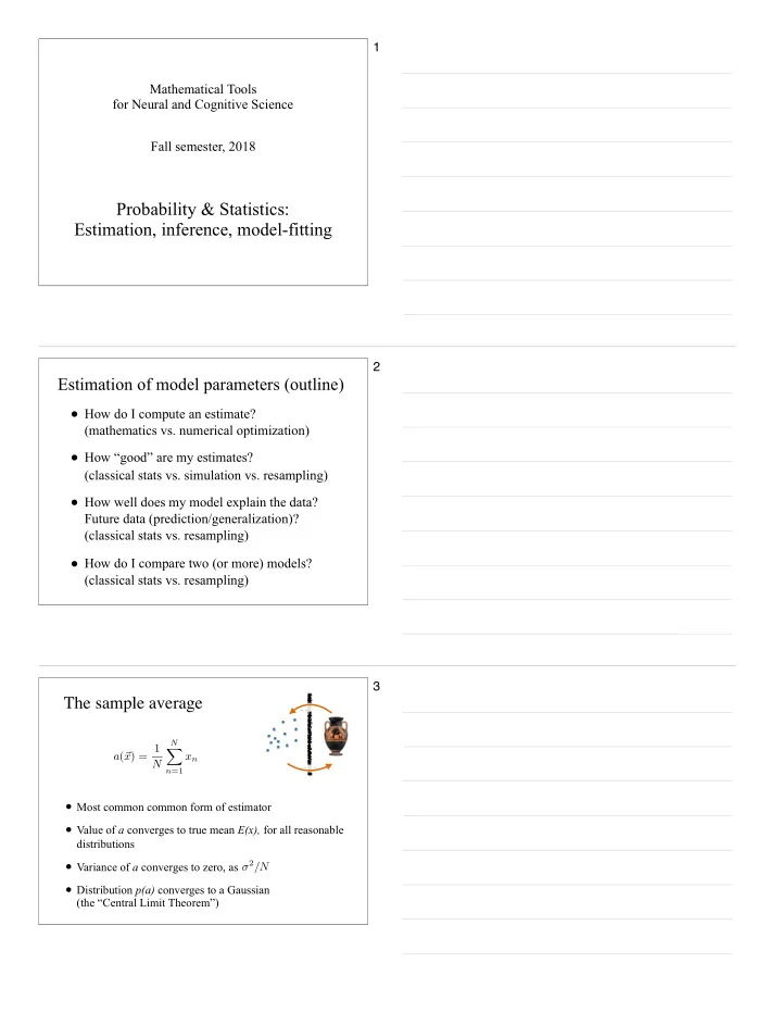
• Most common common form of estimator
• Value of a converges to true mean E(x), for all reasonable

distributions

• Variance of a converges to zero, as
• Distribution p(a) converges to a Gaussian 


(the “Central Limit Theorem”)

The sample average

a(~ x) = 1 N

N

X

n=1

xn

Mea Inf

3

SLIDE 2

The Gaussian

• parameterized by mean and SD (position / width)
• product of two Gaussians is Gaussian! [easy]
• sum of Gaussian RVs is Gaussian! [moderate]
• central limit theorem: sum of many RVs is Gaussian! [hard]

4

−4 −3 −2 −1 1 2 3 4 50 100 150 200 250 300 350 400 450 500 (u+u+u+u)/sqrt(4) −4 −3 −2 −1 1 2 3 4 50 100 150 200 250 104 samples of uniform dist −4 −3 −2 −1 1 2 3 4 100 200 300 400 500 600 10 u’s divided by sqrt(10) −4 −3 −2 −1 1 2 3 4 50 100 150 200 250 300 350 400 450 (u+u)/sqrt(2)

Central limit for a uniform distribution...

10k samples, uniform density (sigma=1)

5

0.2 0.4 0.6 0.8 1 1000 2000 3000 4000 5000 6000

• ne coin

0.2 0.4 0.6 0.8 1 1000 2000 3000 4000 avg of 4 coins 0.2 0.4 0.6 0.8 1 500 1000 1500 2000 avg of 16 coins 0.2 0.4 0.6 0.8 1 500 1000 1500 2000 avg of 64 coins 0.2 0.4 0.6 0.8 1 500 1000 1500 2000 2500 avg of 256 coins

Central limit for a binary distribution...

6

SLIDE 3

true mean: [0 0.8] true cov: [1.0 -0.25

• 0.25 0.3]

sample mean: [-0.05 0.83] sample cov: [0.95 -0.23

• 0.23 0.29]

700 samples Measurement (sampling) Inference true density

7

Point Estimates

• Estimator: Any function of the data, intended to provide

an estimate of the true value of a parameter

• Statistically-motivated estimators:
• Maximum likelihood (ML):
• Max a posteriori (MAP):
• Bayes estimator:
• Bayes least squares:


(special case) ˆ x(~ d) = arg min

ˆ x E

⇣ L(x − ˆ x)|~ d ⌘

8

Estimator quality: Bias & Variance

• Mean squared error = bias^2 + variance
• Bias is difficult to assess (requires knowing the “true”

value). Variance is easier.

• Classical statistics generally aims for an unbiased

estimator, with minimal variance (“MVUE”).

• The MLE is asymptotically unbiased (under fairly

general conditions), but this is only useful if

• the likelihood model is correct
• the optimum can be computed
• you have lots of data
• More general view: estimation is about trading off bias

and variance, through model selection, “regularization”,

• r Bayesian priors…

9

SLIDE 4

• Binomial:





• Poisson:

ML Estimates - discrete

p nhead | m, phead

( ) =

m n ⎛ ⎝ ⎜ ⎞ ⎠ ⎟ phead

n

1− phead

( )

m−n

ˆ phead = n m p k | λ

( ) = λ ke−k

k! ˆ λ = k 10

The N independent samples are ML estimates are x1,x2,!xN ˆ µ = xi

i=1 N

∑

N ˆ σ 2 = xi − x

( )

2 i=1 N

∑

N biased!

ML Estimates - continuous

11

Example: Estimate the bias of a coin

12

SLIDE 5

13

Bayes’ Rule and Estimation

p(parameter value |data) = p(data | parameter value)p(parameter value) p(data)

Posterior Prior Likelihood Nuisance normalizing term

14

Likelihood: 1 head Likelihood: 1 tail

15

SLIDE 6

More heads More tails

T=0 1 2 3 2 3 1 H=0

Posteriors, p(H,T|x), assuming prior p(x)=1

16

example

infer whether a coin is fair by flipping it repeatedly here, x is the probability of heads (50% is fair) y1...n are the outcomes of flips Consider three different priors: suspect fair suspect biased no idea

17

prior fair prior biased prior uncertain X likelihood (heads) = posterior

18

SLIDE 7

previous posteriors X likelihood (heads) = new posterior

19

previous posteriors X likelihood (tails) = new posterior

20

Posteriors after observing 75 heads, 25 tails àprior differences are ultimately overwhelmed by data

21

SLIDE 8

PDFs CDFs, and 95% confidence intervals

10H / 5T 20H / 10T 2H / 1T .975 .025 .19 .93 .49 .80

Confidence intervals

22

Statistical Rethinking, Richard McElreath

Classical “frequentist” statistical tests

23

Classical/frequentist approach - z

• H1: NZT improves IQ
• Null: H0: it does nothing
• In the general population,

IQ is known to be distributed normally with

• µ = 100
• σ = 15
• We give the drug to 30

people and test their IQ. 24

SLIDE 9

• µ = 100 (Population mean)
• σ = 15 (Population standard deviation)
• N = 30 (Sample contains scores from

30 participants)

• x = 108.3 (Sample mean)
• z = (x – µ)/SE = (108.3-100)/SE

(Standardized score)

• SE = σ / √N = 15/√30 = 2.74
• Error bar/CI: ±2 SE
• z = 8.3/2.74 = 3.03
• p = 0.0012
• Significant?
• One- vs. two-tailed test

The z-test

25

• µ = 100 (Population mean)
• σ = 15 (Population standard

deviation)

• N = 30 (Sample contains scores from

30 participants)

• x = 104.2 (Sample mean)
• z = (x – µ)/SE = (104.2-100)/SE
• SE = σ / √N = 15/√30 = 2.74
• z = 4.2/2.74 = 1.53
• p = 0.061
• Significant?

What if the measured effect of NZT had been half that?

26

Significance levels

• Are denoted by the Greek letter α.
• In principle, we can pick anything that we

consider unlikely.

• In practice, the consensus is that a level of 0.05 or

1 in 20 is considered as unlikely enough to reject H0 and accept the alternative.

• A level of 0.01 or 1 in 100 is considered “highly

significant” or really unlikely.

27

SLIDE 10

Does NZT improve IQ scores or not?

Reality Yes No Significant? Yes No

Correct Type I error α-error False alarm Correct Type II error β-error Miss

28

Test statistic

• We calculate how far the observed value of the

sample average is away from its expected value.

• In units of standard error.
• In this case, the test statistic is
• Compare to a distribution, in this case z or N(0,1)

z = x − µ SE = x − µ σ / N

29

Common misconceptions

Is “Statistically significant” a synonym for:

• Substantial
• Important
• Big
• Real

Does statistical significance gives the

• probability that the null hypothesis is true
• probability that the null hypothesis is false
• probability that the alternative hypothesis is true
• probability that the alternative hypothesis is false

Meaning of p-value. Meaning of CI.

30

SLIDE 11

Student’s t-test

• σ not assumed known
• Use



 


• Why N-1? s is unbiased (unlike ML version), i.e.,

• Test statistic is





• Compare to t distribution for CIs and NHST
• “Degrees of freedom” reduced by 1 to N-1

s2 = xi − x

( )

2 i=1 N

∑

N −1

E(s2) = σ 2 t = x − µ0 s / N

31

The t distribution approaches the normal distribution for large N

x (z or t)

Probability

32

The z-test for binomial data

• Is the coin fair?
• Lean on central limit theorem
• Sample is n heads out of m tosses
• Sample mean:
• H0: p = 0.5
• Binomial variability (one toss):
• Test statistic:





• Compare to z (standard normal)
• For CI, use

ˆ p = n / m

σ = pq, where q = 1− p

z = ˆ p − p0 p0q0 / m

±zα /2 ˆ p ˆ q / m

33

SLIDE 12

Many varieties of frequentist univariate tests

• goodness of fit
• test of independence
• test a variance using
• F to compare variances (as a ratio)
• Nonparametric tests (e.g., sign, rank-order, etc.)

χ 2 χ 2 χ 2

34

Bootstrapping

• “The Baron had fallen to the bottom of a deep lake.

Just when it looked like all was lost, he thought to pick himself up by his own bootstraps” 


[Adventures of Baron von Munchausen, by Rudolph Erich Raspe]

• A (re)sampling method for computing estimator

distribution (incl. stdev error bars or confidence intervals)

• Idea: instead of running experiment multiple times,

resample (with replacement) from the existing

• data. Compute an estimate from each of these

“bootstrapped” data sets.

35

[Efron & Tibshirani ’98] [New York Times, 27 Jan 1987] Histogram of bootstrap estimates:

0.2 0.4 0.6 0.8 1 200 400 600 800 1000 1200 1400 Boostrapped Original 95% conf

=> with 95% confidence,

36

SLIDE 13

[Efron & Tibshirani ’98]

37

data { ⃗ x n} probabilistic model pθ( ⃗ x )

Measurement Inference

38

• Estimator: Any function of the data, intended to provide

an estimate of the true value of a parameter

• The most common estimator is the sample average, used

to estimate the true mean of a distribution.

• Statistically-motivated estimators:
• Maximum likelihood (ML):
• Max a posteriori (MAP):
• Bayes estimator:

Point Estimates

ˆ x(~ d) = arg min

ˆ x E

⇣ L(x − ˆ x)|~ d ⌘

39

SLIDE 14

40

P(x|N) P(x|S)

Signal Detection Theory For equal, unimodal, symmetric distributions, ML decision rule is a threshold function.

“S” “N”

x

41

Signal Detection Theory: Potential outcomes

threshold

Tumor present Tumor absent Doctor responds “yes” Doctor responds “no”

P(x|N) P(x|S) P(x|N) P(x|S) x x

correct reject false alarm hit miss

42

SLIDE 15

N S+N Internal response Probability

d’

Internal response: probability of occurrence curves

N: noise only (tumor absent) S+N: signal plus noise (tumor present) Discriminability (“d-prime”) is the normalized separation between the two distributions

d’ = separation spread

43

Signal Detection Theory: discriminability (d’)

44

N S+N Criterion Internal response Probability Say “yes” Say “no”

• Vision
• Detection (something vs. nothing)
• Discrimination (lower vs greater level of: intensity, contrast, depth, slant, size,

frequency, loudness, ...

• Memory (internal response = trace strength = familiarity)
• Neurometric function/discrimination by neurons (internal


response = spike count)

Example applications of SDT

45

SLIDE 16

Criterion

Internal response Probability Criterion

Say “yes” Say “no” Distribution of internal responses when no tumor Distribution of internal responses when tumor present

46

Signal Detection Theory: Criterion

47

SDT: Gaussian case

N S+N x Probability

′ d

c

c = z[p(CR)] ′ d = z[p(H)]+ z[p(CR)] = z[p(H)]− z[p(FA)]

z[p(CR)] z[p(H)]

G(x;µ,σ ) = 1 2πσ e−(x−µ)2/2σ 2 β = p(x = c | S + N) p(x = c | N) = e−(c− ′

d )2/2

e−c2/2

48

SLIDE 17

Internal response Probability

False Alarms Hits 1 1

ROC (Receiver Operating Characteristic)

Criterion #1

49

Internal response Probability

False Alarms Hits 1 1

Criterion #2

ROC (Receiver Operating Characteristic)

50

Internal response Probability

False Alarms Hits 1 1

Criterion #3

ROC (Receiver Operating Characteristic)

51

SLIDE 18

Internal response Probability

False Alarms Hits 1 1

Criterion #4

ROC (Receiver Operating Characteristic)

52

ROC (Receiver Operating Characteristic)

53

N S+N z[p(FA)] z[p(H)]

ROC: Gaussian case

Probability c

54

SLIDE 19

Decision/classification in multiple dimensions

• Data-driven:
• Fisher Linear Discriminant (FLD) - maximize d’
• Support Vector Machine (SVM) - maximize margin
• Statistical:
• ML/MAP/Bayes under a probabilistic model
• e.g.: Gaussian, equal covariance (same as FLD)
• e.g.: Gaussian, unequal covariance (QDA)
• Examples:
• Visual gender identification
• Neural population decoding

55

mean: [0.2, 0.8] cov: [1.0 -0.3;

• 0.3 0.4]

Multi-D Gaussian densities

56

Find unit vector ˆ

w (“discriminant”) that best separates two distributions

Linear Classifier

Simplest choice: difference of means

57

SLIDE 20

max

ˆ w

⇥ ˆ wT (µA − µB) ⇤2 [ ˆ wT CA ˆ w + ˆ wT CB ˆ w] ˆ w = D−1V T (µA − µB), where V D2V T = CA + CB

Fisher Linear Discriminant

58

Support Vector Machine

find largest m, and { ˆ w, b} s.t. ci( ˆ wT~ xi − b) ≥ m, ∀ i

ˆ w

ci = 1 ci = −1

Maximize the “margin” (gap between data sets)

59

Gaussian ML classifier

[figure: Pagan et al. 2016]

For equal covariances: Linear For different covariances: Quadratic (three possible geometries)

60

SLIDE 21

• 200 face images (100 male, 100 female)
• Adjusted for position, size, intensity/contrast
• Labeled by 27 human subjects

[Graf & Wichmann, NIPS*03]

Example: Gender identification

61

Linear classifiers

SVM RVM Prot FLD trained

• n

→ W true data → W subj data

w w

SVM RVM Prot FLD

Four linear classifiers trained on subject data

62

Model validation/testing

• Cross-validation: Subject responses [%

correct, reaction time, confidence] are explained

• very well by SVM
• moderately well by RVM / FLD
• not so well by Prot
• Curse of dimensionality strongly limits this
• result. A more direct test: Synthesize
• ptimally discriminable faces...

63

SLIDE 22

ε=−21 ε=−14 ε=−7 ε=0 ε=7 ε=14 ε=21 SVM RVM Prot FLD

Add classifier Subtract classifier

[Wichmann, Graf, Simoncelli, Bülthoff, Schölkopf, NIPS*04]

64

50 100

% Correct Amount of classifier image added/subtracted (arbitrary units)

1.0 2.0 4.0 8.0 0.5 0.25

SVM RVM Proto FLD

[Wichmann, Graf, Simoncelli, Bülthoff, Schölkopf, NIPS*04]

65 66

SLIDE 23

Independent Poisson responses 


[e.g., Seung & Sompolinsky, 1993]

• 5

10 15 20 25 30 0.50 0.75 0.90 0.95 0.99 Orientation difference (degrees) Probability correct ELD CB-ELD PID

a

N = 20 from 60 SVM shuffled-SVM

Graf, Kohn, Jazayeri, Movshon, 2011

shuffled-SVM indep-Poisson

Tuning curves,

s hn(s)

Population decoding

67

• Is the coin fair? Compared to what?
• Point hypotheses:

Bayesian Model Comparison

M1 : p = p1 = 0.5 M2 : p = p2 = 0.6 p(M1 | D) = p(D | M1)P(M1) p(D) = p(D | M1)P( p1) p(D)

Assuming equal priors over models the Bayes factor is

p(M1 | D) p(M2 | D) = p(D | M1)P(M1) p(D | M2)P(M2) = p(D | M1)P( p1) p(D | M2)P( p2) 68

• Is the coin fair? Compared to what?
• Alternative hypothesis:

Bayesian Model Comparison

M1 : p = p1 = 0.5 M2 : p ≠ 0.5 p(M2 | D) = p(D | M2)p(M2) p(D) = p( pcoin | D)p( pcoin)dpcoin

1

∫

= p(D | M2, pcoin)p( pcoin)dpcoin

1

∫

P(M2) p(D)

Compute Bayes factor as before.

69

SLIDE 24

Continuous/Gaussian: Localization

I find that . Is that convincing? Is the apparent bias real?

x ≠ 0 70

Continuous/Gaussian: Localization

Take N independent samples from the distribution, these act like draws from N independent, identically distributed (IID) RVs: X1, X2,!X N

71

Continuous/Gaussian: Localization

The N independent samples are ML estimates are x1,x2,!xN ˆ µ = xi

i=1 N

∑

N ˆ σ 2 = xi − x

( )

2 i=1 N

∑

N −1 72

SLIDE 25

Continuous/Gaussian: Localization

MAP estimates of the mean are based on the posterior, a product of Gaussians (assuming a Gaussian) prior. Thus there is shrinkage toward the prior. Model comparison for hypotheses about the mean (variance assumed known) are similar to the binomial example.

73

The Gaussian

• parameterized by mean and stdev (position / width)
• joint density of two indep Gaussian RVs is circular! [easy]
• product of two Gaussian dists is Gaussian! [easy]
• conditionals of a Gaussian are Gaussian! [easy]
• sum of Gaussian RVs is Gaussian! [moderate]
• all marginals of a Gaussian are Gaussian! [moderate]
• central limit theorem: sum of many RVs is Gaussian! [hard]
• most random (max entropy) density with this variance! [moderate]

74

Completing the square shows that this posterior is also Gaussian, with

(average, weighted by inverse variances!)

∝

Product of Gaussian distributions is Gaussian

75

SLIDE 26

Completing the square shows that this posterior is also Gaussian, with

(average, weighted by inverse variances!)

p(x|y) ∝ p(y|x)p(x) ∝ e

− 1

2



1 σ2 n (x−y)2

• e

− 1

2



1 σ2 x (x−µx)2

• =

e

− 1

2

✓

1 σ2 n + 1 σ2 x

◆ x2−2 ✓

y σ2 n + µx σ2 x

◆ x+...

• Product of Gaussian distributions is Gaussian

76

The Gaussian

• parameterized by mean and stdev (position / width)
• joint density of two indep Gaussian RVs is circular! [easy]
• product of two Gaussian dists is Gaussian! [easy]
• conditionals of a Gaussian are Gaussian! [easy]
• sum of Gaussian RVs is Gaussian! [moderate]
• all marginals of a Gaussian are Gaussian! [moderate]
• central limit theorem: sum of many RVs is Gaussian! [hard]
• most random (max entropy) density with this variance! [moderate]

77

mean: [0.2, 0.8] cov: [1.0 -0.3;

• 0.3 0.4]

Multi-D Gaussian densities

78

SLIDE 27

~ x ∼ N(~ µ, C), let P = C−1 Gaussian, with:

Conditional:

p(x1|x2 = a) ∝ e− 1

2[P11(x1−µ1)2+2P12(x1−µ1)(a−µ2)+...]

= e− 1

2[P11x2 1+2(P12(a−µ2)−P11µ1)x1+...]

= e

− 1

2

⇣ x1−µ1+ P12

P11 (a−µ2)

⌘ P11 ⇣ x1−µ1+ P12

P11 (a−µ2)

⌘ +...

Marginal:

Gaussian, with:

p(x1) = Z p(~ x) dx2 (the “precision” matrix)

[on board]

79

ˆ u z = ˆ uT~ x µz = ˆ uT ~ µx 2

z

= ˆ uT Cxˆ u z p(z)

Generalized marginals of a Gaussian

x1 x2 w

is Gaussian, with:

80

Bivariate statistics

• Covariance of X and Y:

• Correlation of X and Y:



 


• Unbiased estimators from samples:

Cov(X,Y) = E X − µX

( ) Y − µY ( )

( )

ρ XY = Cov(X,Y) σ Xσ Y

rxy = xi − x

( ) yi − y ( )

i=1 N

∑

N −1

( )sxsy

= xi − x

( ) yi − y ( )

i=1 N

∑

xi − x

( )

2 i=1 N

∑

yi − y

( )

2 i=1 N

∑

sxy = xi − x

( ) yi − y ( )

i=1 N

∑

N −1

( )

81

SLIDE 28

Correlation: summary of data cloud shape

+ + -

• 82

Correlation captures dependency, but not “shape”

83

Correlation and regression

TLS (largest eigenvector) Least-squares regression

“Regression to the mean”

84

SLIDE 29

−5 5 −5 5 corr=−0.80 −5 5 −5 5 corr=−0.40 −5 5 −5 5 corr=0.00 −5 5 −5 5 corr=0.40 −5 5 −5 5 corr=0.80

Correlation and regression

85

Variance partitioning and model assessment

SStotal = yi − y

( )

2 i=1 N

∑

= SSexplained + SSresidual SSexplained = ˆ yi − y

( )

2 i=1 N

∑

SSresidual = ˆ yi − yi

( )

2 i=1 N

∑

• Coeff. of determination r 2 =

SSexplained SStotal 86

Correlation between variables does not uniquely indicate their relationship

87

SLIDE 30

https://www.autodeskresearch.com/publications/samestats

More extreme examples !

88

Statistical independence a stronger assumption uncorrelatedness

⇒ All independent variables are uncorrelated ⇒ Not all uncorrelated variables are independent:

r =

Independence implies uncorrelated, but uncorrelated doesn’t imply independent!

89

Null Hypothesis: Distribution of normalized dot product of pairs of Gaussian vectors in N dimensions:

N=3 N=8

−1 −0.5 0.5 1 0.2 0.4 0.6 0.8 1 1.2 −1 −0.5 0.5 1 0.2 0.4 0.6 0.8 1 1.2 −1 −0.5 0.5 1 0.5 1 1.5

N=4 N=16

−1 −0.5 0.5 1 0.02 0.04 0.06 0.08 −1 −0.5 0.5 1 0.01 0.02 0.03 0.04 0.05 −1 −0.5 0.5 1 0.005 0.01 0.015 0.02 0.025

N=32 N=64

Lack of correlation is favored in N>3 dimensions

(1 − d2)

N−3 2

90

SLIDE 31

sin(theta)^(N-2)

1 2 3 0.5 1 1.5 2 1 2 3 0.5 1 1.5 1 2 3 0.2 0.4 0.6 0.8 1 1 2 3 0.2 0.4 0.6 0.8 1 2 3 0.2 0.4 0.6 0.8 1 2 3 0.2 0.4 0.6 0.8 1

Distribution of angles of pairs of Gaussian vectors

2D 3D 4D 6D 10D 18D

91

Sociology doctorates awarded (US) Worldwide non-commercial space launches

Worldwide non-commercial space launches

correlates with

Sociology doctorates awarded (US)

Sociology doctorates awarded (US) Worldwide non-commercial space launches 1997 1998 1999 2000 2001 2002 2003 2004 2005 2006 2007 2008 2009 1997 1998 1999 2000 2001 2002 2003 2004 2005 2006 2007 2008 2009 500 Degrees awarded 550 Degrees awarded 600 Degrees awarded 650 Degrees awarded 700 Degrees awarded 40 Launches 50 Launches 30 Launches 60 Launches tylervigen.com Number of people killed by venomous spiders Spelling Bee winning word

Letters in Winning Word of Scripps National Spelling Bee

correlates with

Number of people killed by venomous spiders

Number of people killed by venomous spiders Spelling Bee winning word 1999 2000 2001 2002 2003 2004 2005 2006 2007 2008 2009 1999 2000 2001 2002 2003 2004 2005 2006 2007 2008 2009 0 deaths 5 deaths 10 deaths 15 deaths 5 letters 10 letters 15 letters tylervigen.com Bedsheet tanglings Cheese consumed

Per capita cheese consumption

correlates with

Number of people who died by becoming tangled in their bedsheets

Bedsheet tanglings Cheese consumed 2000 2001 2002 2003 2004 2005 2006 2007 2008 2009 2000 2001 2002 2003 2004 2005 2006 2007 2008 2009 200 deaths 400 deaths 600 deaths 800 deaths 28.5lbs 30lbs 31.5lbs 33lbs tylervigen.com

Nevertheless,

• ne can find

correlation if

• ne looks for it!

http://www.tylervigen.com/spurious-correlations

92

Correlation does not imply causation

• Beware selection bias
• Correlation does not provide a direction for causality.

For that, you need additional (temporal) information.

• More generally, correlations are often a result of

hidden (unmeasured, uncontrolled) variables…

Example: conditional independence:

p(A,B | H) = p(A | H) p(B | H)

A B H [on board: In Gaussian case, connections are explicit in the Precision Matrix]

+ +

93

SLIDE 32

Another example: Simpson’s paradox

+

• A

B H +

94

Milton Friedman’s Thermostat

O = outside temperature (assumed cold) I = inside temperature (ideally, constant) E = energy used for heating Statistical observations:

• O and I uncorrelated
• I and E uncorrelated
• O and E anti-correlated

Some nonsensical conclusions:

• O and E have no effect on I, so shut off heater to save money!
• I is irrelevant, and can be ignored. Increases in E cause decreases in O.
• O

I E

+ +

• O

I E

True interactions: Statistical interactions, P=C-1:

Statistical summary cannot replace scientific reasoning/experiments!

95

Summary: Correlation misinterpretations

• Correlation does not imply data lie on a line

(subspace), with noise perturbations

• Correlation => dependency, but lack of correlation

does not imply independence

• Correlation does not imply causation (temporally, or

by direct influence/connection)

• Correlation is a descriptive statistic, and cannot

replace the need for scientific reasoning/experiment!

96

SLIDE 33

• Optimization failures (e.g., local minima)


[convex relaxation, test with simulations]

• Overfitting (too many params, not enough data)

[use cross-validation to select complexity, or to control regularization]

• Experimental variability (due to finite/noisy

measurements) [use math/distributional assumptions, or simulations, or bootstrapping]

• Model failures

Taxonomy of model-fitting errors

97

statAnMod - 9/12/07 - E.P. Simoncelli

Optimization...

Smooth (C2) Convex Quadratic Closed-form, and unique Iterative descent, (possible local minima) Iterative descent, unique Heuristics, exhaustive search, (pain & suffering)

98 99

SLIDE 34

Cross-validation

(1) Randomly partition data into a “training” set, and a “test” set. (2) Fit model to training set. Measure error on test set. (3) Repeat (many times) (4) Choose model that minimizes the cross-validated (test) error

A resampling method for constraining a model. Widely used to identify/avoid over-fitting.

5 10 15 20 10

−2

10 10

2

10

4

10

6

polynomial degree MSE fit error x−val error true degree true error

train error test error

Using cross-validation to select the degree of a polynomial model:

100

arg min

~

• ||~

y − X~ ||2 arg min

~

• ||~

y − X~ ||2 + ||~ ||2

Ridge regression

(a.k.a. Tikhonov regularization)

Equivalent formulation: MAP estimate, assuming Gaussian likelihood & prior! Ordinary least squares regression: “Regularized” least squares regression: Choose lambda by cross-validation:

0.2 0.4 0.6 0.8 1 −2 −1 1 2 3 4 5 data LS reg Ridge reg

7th-order polynomial regression:

ˆ ridge = (XT X + I)−1XT~ y

101

5 10 15 20 25 0.0 0.2 0.4 0.6 0.8 λ Linear MSE Ridge MSE Ridge Bias^2 Ridge Var

Linear regression: Squared bias ≈ 0.006 Variance ≈ 0.627

• Pred. error ≈ 1 + 0.006 + 0.627
• Pred. error ≈ 1.633

Ridge regression, at its best: Squared bias ≈ 0.077 Variance ≈ 0.403

• Pred. error ≈ 1 + 0.077 + 0.403
• Pred. error ≈ 1.48

from http://www.stat.cmu.edu/~ryantibs/datamining/

102

SLIDE 35

arg min

~

• ||~

y − X~ ||2 + X

k

|k|

L1 regularization

(a.k.a. least absolute shrinkage and selection operator - LASSO)

L1 norm (still convex)

Using an absolute error regularization term promotes binary selection of regressors:

From Hastie, Tibshirani, Wainwright 2015

103

Solving for LASSO in 1D: soft-thresholding arg min

β ||~

y − ~ x||2 + || assume ||~ x||2 = 1

[solution on board]

~ yT~ x

β

λ/2 λ/2

ˆ βOLS ˆ βLASSO ˆ βridge

104

“relaxed LASSO”

Bias reduction using the “relaxed LASSO”: Re-solve for non-zero coefficients after eliminating unused regressors

LASSO

105

SLIDE 36

LASSO vs. Ridge regression

0.0 0.2 0.4 0.6 0.8 1.0 −5 5 10 Coefficients hs college college4 not−hs funding

Lasso

0.0 0.2 0.4 0.6 0.8 1.0 −5 5 10 Coefficients hs college college4 not−hs funding

Ridge Regression kˆ βk1/k˜ βk1 kˆ βk2/k˜ βk2 Table 2.1 Crime data: Crime rate and five predictors, for N = 50 U.S. cities. city funding hs not-hs college college4 crime rate 1 40 74 11 31 20 478 2 32 72 11 43 18 494 3 57 70 18 16 16 643 4 31 71 11 25 19 341 5 67 72 9 29 24 773 . . . . . . . . . . . . . . . 50 66 67 26 18 16 940

[From Hastie, Tibshirani, Wainwright 2015]

← λ

106

• K-Means (Lloyd, 1957)

Clustering

• “Soft-assignment” version of K-means

(a form of Expectation-Maximization - EM)

• In general, alternate between:

1) Estimating cluster assignments 2) Estimating cluster parameters

• Coordinate descent: converges to (possibly local) minimum
• Need to choose K (number of clusters)

107

• Estimating cluster assignments: given class centers,

assign each point to closest one.

y .

• n
• 0.0

0.5 1.0 1.5 −0.5 0.0 0.5 1.0 1.5

• Estimating cluster parameters: given assignments, re-

estimate the centroid of each cluster. K-Means

Soap bubbles:

108

SLIDE 37

K-means example

Here Xi ∈ R2, n = 300, and K = 3

• ●
• −0.5

0.0 0.5 1.0 1.5 0.0 0.5 1.0 1.5 2.0 Initial centers

• ●
• −0.5

0.0 0.5 1.0 1.5 0.0 0.5 1.0 1.5 2.0 Iteration 1

• ●
• −0.5

0.0 0.5 1.0 1.5 0.0 0.5 1.0 1.5 2.0 Iteration 2

• ●
• −0.5

0.0 0.5 1.0 1.5 0.0 0.5 1.0 1.5 2.0 Iteration 3

• ●
• −0.5

0.0 0.5 1.0 1.5 0.0 0.5 1.0 1.5 2.0 Iteration 9

• [from R. Tibshirani, 2013]

109

• 0.0

0.5 1.0 1.5 −0.5 0.0 0.5 1.0 1.5 WCV = 25.9

• 0.0

0.5 1.0 1.5 −0.5 0.0 0.5 1.0 1.5 WCV = 18.1

• 0.0

0.5 1.0 1.5 −0.5 0.0 0.5 1.0 1.5 WCV = 24.3

• Warning: Initialization matters…

Three solutions obtained with different random starting points:

[from R. Tibshirani, 2013]

110

Non-convex/non-round-shaped clusters: Standard K-means fails! Clusters with different densities

Picture courtesy: Christof Monz (Queen Mary, Univ. of London)

K-means failures

111

SLIDE 38

ML for discrete mixture of Gaussians

= assignment probability = mean/covariance of class n Intuition: alternate between maximizing these two sets of variables (“coordinate descent”)

p(~ xn|ank, ~ µk, Λk) ∝ X

k

ank p |Λk| e−(~

xn−~ µk)T Λ−1

k (~

xn−~ µk)/2

ank {~ µk, Λk}

112

[wikipedia]

113

Standard solution:

• 1. Threshold to find segments containing spikes
• 2. Reduce dimensionality of segments using PCA
• 3. Identify spikes using clustering (e.g., K-means)

Note: Fails for overlapping spikes!

Application to neural “spike sorting”

114

SLIDE 39

A synchronous spiking superposition for various time shifts C B

+ =

PC 1 projection PC 2 projection

+ =

D PC 1 projection

0 ms +0.1 ms

• 0.15 ms

+0.45 ms

Failures of clustering for near-synchronous spikes

[Pillow et. al. 2013]

115

PC 2

hit miss false positive 2

a b c d

Simulated data [Quiroga et. al. 2004]

PC 1 PC 1

clustering (K-means) CBP

[Ekanadham et al, 2014]

116 Linear systems / Fourier analysis Linear algebra Machine learning & pattern recognition Statistics Optimization Data analysis & Modeling 117

SLIDE 40

mathematical manipulation g e

• m

e t r i c r e a s

• n

i n g c

• m

p u t e r i m p l e m e n t a t i

• n

118