The Fourier Transform I Image Analysis The Fourier transform Those - - PowerPoint PPT Presentation

SLIDE 1

Image Analysis

The Fourier transform Niclas Börlin niclas.borlin@cs.umu.se

Department of Computing Science Umeå University

January 30, 2009

Niclas Börlin (CS, UmU) The Fourier transform January 30, 2009 1 / 30

The Fourier Transform I

Those who combine a theoretical knowledge of Fourier transform properties with a knowledge of their physical interpretation are well prepared to approach most image-processing problems. . . , the time spent becoming familiar with the Fourier transform is well invested — Kenneth R. Castleman

Niclas Börlin (CS, UmU) The Fourier transform January 30, 2009 2 / 30

The Fourier transform I

In 1822, Joseph Fourier published some astonishing results:

1

All periodical functions can be expressed as a series of sines and cosines.

2

All functions that enclose a finite area can be expressed as a series of sines and cosines. The Fourier series for a periodic function f(t), of a continous variable t, with period T is f(t) =

∞

• n=−∞

cnej 2πn

T t,

where j = √ −1, ejθ = cos θ + j sin θ, and cn = 1 T T/2

−T/2

f(t)e−j 2πn

T tdt

are the Fourier coefficients of f(t).

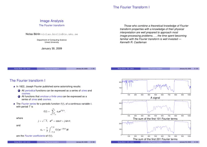
Niclas Börlin (CS, UmU) The Fourier transform January 30, 2009 3 / 30 100 200 300 400 500 600 700 800 900 1000 100 200

A signal

100 200 300 400 500 600 700 800 900 1000 100 200

The sum of the first 101 Fourier terms

100 200 300 400 500 600 700 800 900 1000 100 200

The sum of the first 201 Fourier terms

Niclas Börlin (CS, UmU) The Fourier transform January 30, 2009 4 / 30

SLIDE 2

The Fourier transform

The continuous Fourier transform of a complex-valued function f(t) is defined as F{f(t)} = F(s) = ∞

−∞

f(t)e−j2πstdt. Its inverse is defined as F−1{F(s)} = f(t) = ∞

−∞

F(s)ej2πstds. The Fourier transform for a function is unique. The functions f(t) and F(s) are called a Fourier transform pair.

Niclas Börlin (CS, UmU) The Fourier transform January 30, 2009 5 / 30

The Fourier transform of a Gaussian

Given f(t) = e−πt2 we have F(s) = ∞

−∞

e−πt2e−j2πstdt = ∞

−∞

e−π(t2+jst)dt. Multiply the right hand side by e−πs2eπs2: F(s) = e−πs2 ∞

−∞

eπs2e−π(t2+jst)dt = e−πs2 ∞

−∞

e−π(t2+jst−s2)dt = e−πs2 ∞

−∞

e−π(t+js)2dt = e−πs2 ∞

−∞

e−πu2du = e−πs2. Thus the Fourier transform of a Gaussian is another Gaussian.

Niclas Börlin (CS, UmU) The Fourier transform January 30, 2009 6 / 30

When does the Fourier transform exist?

The Fourier transform does not exist for all functions. However, the Fourier transform always exists if ∞

−∞

|f(t)|dt < ∞ and f(t) is continuous or f(t) has a finite number of discontinuities. Such a function is called transient. Thus, the Fourier transform exists for all signals (images) that are possible to represent in a computer!

Niclas Börlin (CS, UmU) The Fourier transform January 30, 2009 7 / 30

The spatial domain vs. the frequency domain

From the Euler formula ejθ = cos θ + j sin θ we see that all functions with a well-defined Fourier transform can be re-written as a sum of sines and cosines of different frequencies. This is why we say that the Fourier transform takes us from the spatial domain (or the time domain) to the frequency domain.

Niclas Börlin (CS, UmU) The Fourier transform January 30, 2009 8 / 30

SLIDE 3

Properties of complex functions

In general, the Fourier transform of a real function is complex. A complex function F(u) = R(u) + jI(u) may be expressed as F(u) = |F(u)|e−jφ(u), where |F(u)| =

• R2(u) + I2(u),

is known as the spectrum and φ(u) = tan−1 I(u) R(u) is known as the phase angle. The Power spectrum or Power spectral density is defined as P(u) = |F(u)|2.

Niclas Börlin (CS, UmU) The Fourier transform January 30, 2009 9 / 30

Impulses

A Unit impulse of a continous variable t located at t = 0, is defined as δ(t) = ∞ if t = 0

• therwise .

Furthermore, δ(t) satisfies ∞

−∞

δ(t)dt = 1. The unit impulse δ(t) is called the Dirac Delta function, even though it is not a proper function.

Niclas Börlin (CS, UmU) The Fourier transform January 30, 2009 10 / 30

Sifting

The Dirac delta has the following important sifting property ∞

−∞

f(t)δ(t)dt = f(0)

• r

∞

−∞

f(t)δ(t − t0)dt = f(t0), assuming that f(t) is continous at t0. This means that F{δ(t − t0)} = ∞

−∞

δ(t − t0)e−j2πstdt = e−j2πst0 and F{δ(t − 0)} = ∞

−∞

δ(t − t0)e−j2πstdt = e−j2πs0 = 1.

Niclas Börlin (CS, UmU) The Fourier transform January 30, 2009 11 / 30

Impulse train — the Shah function

An Impulse train is a sum of infinitely many periodic impulses ∆T apart s∆T(t) =

∞

• n=−∞

δ(t − n∆T). The expression s∆T(t) is sometimes called the Shah function or sampling function. We will use impulse trains later during sampling.

Niclas Börlin (CS, UmU) The Fourier transform January 30, 2009 12 / 30

SLIDE 4

The box and sinc functions

Another function important for sampling is the box function f(t) = A if |t| ≤ W/2

• therwise

whith its fourier transform F(s) = AW sin(πsW) πsW = AW sinc(sW), where the sinc function is defined as sinc(x) = sin πx πx .

Niclas Börlin (CS, UmU) The Fourier transform January 30, 2009 13 / 30

The symmetry of the Fourier transform

The forward and inverse Fourier transforms differs by only the sign of the exponential. Thus, if F(s) = F{f(t)}, then F{F(t)} = f(−s). For example, if f(t) is the box function and F(s) = F{f(t)} = AW sinc(sW), then F{F(s)} = F{AW sinc(sW)} = f(−s). Thus, the Fourier transform of a box function is a sinc function, and vice versa.

Niclas Börlin (CS, UmU) The Fourier transform January 30, 2009 14 / 30

Three box functions and their Fourier transforms

f(x) |F(u)|

Niclas Börlin (CS, UmU) The Fourier transform January 30, 2009 15 / 30

Some useful theorems

The Addition theorem: For two functions f(t) and g(t), F{f(t) + g(t)} = F{f(t)} + F{g(t)} = F(s) + G(s). The Shift theorem: If a function f(t) is shifted an amount a, then F{f(t − a)} = e−j2πasF(s). The Similarity theorem: For a function f(t) with Fourier transform F(s), F{f(at)} = 1 |a|F(s/a). Thus, if the function is compressed in one domain it is expanded in the other.

Niclas Börlin (CS, UmU) The Fourier transform January 30, 2009 16 / 30

SLIDE 5

The Fourier transform of the Shah function

The Shah function is periodic with period ∆T s∆T(t) =

∞

• n=−∞

δ(t − n∆T). Thus it can be written as a Fourier series s∆T(t) =

∞

• n=−∞

cnej 2πn

∆T t,

where cn = 1 ∆T ∆T/2

−∆T/2

s∆T(t)e−j 2πn

∆T tdt. Niclas Börlin (CS, UmU) The Fourier transform January 30, 2009 17 / 30

The Fourier transform of the Shah function

The interval [−∆T/2, ∆T/2] contains only the impulse at the

• rigin.

Thus, cn = 1 ∆T ∆T/2

−∆T/2

δ(t)e−j 2πn

∆T tdt =

1 ∆T e0 = 1 ∆T . and s∆T(t) = 1 ∆T

∞

• n=−∞

ej 2πn

∆T t.

We want to find F{s∆T(t)} = 1 ∆T

∞

• n=−∞

F{ej 2πn

∆T t}. Niclas Börlin (CS, UmU) The Fourier transform January 30, 2009 18 / 30

The Fourier transform of the Shah function

We know that F{δ(t − t0)} = e−j2πst0. Thus, by symmetry F{e−j2πtt0} = δ(−s − t0). Substituting −t0 = n/∆T we find that F{ej 2πn

∆T t} = δ(−s + n/∆T) = δ(n/∆T − s) = δ(s − n/∆T).

Thus, F{s∆T(t)} = 1 ∆T

∞

• n=−∞

δ(s − n/∆T). In other words, the Fourier transform of an impulse train with period ∆T is another impulse train with period 1/∆T.

Niclas Börlin (CS, UmU) The Fourier transform January 30, 2009 19 / 30

Convolution and the Convolution theorem

The convolution of two continous functions f(t) and h(t) is defined as f(t) ⋆ h(t) = ∞

−∞

f(τ)h(t − τ)dτ. The Fourier transform of the convolution is F{f(t) ⋆ h(t)} = ∞

−∞

∞

−∞

f(τ)h(t − τ)dτ

• e−j2πstdt

= ∞

−∞

f(τ) ∞

−∞

h(t − τ)e−j2πstdt

• F{h(t−τ)}=H(s)e−j2πst

dτ = H(s) ∞

−∞

f(τ)e−j2πstdτ = H(s)F(s).

Niclas Börlin (CS, UmU) The Fourier transform January 30, 2009 20 / 30

SLIDE 6

Convolution and the Convolution theorem

Thus, a convolution f(t) ⋆ h(t) in the spatial domain corresponds to a multiplication F(s)H(s) in the frequency domain and is written as f(t) ⋆ h(t) ⇔ F(s)H(s). By symmetry, we get f(t)h(t) ⇔ F(s) ⋆ H(s). These two relationships are called the Convolution theorem.

Niclas Börlin (CS, UmU) The Fourier transform January 30, 2009 21 / 30

The two-dimensional Fourier transform

The two dimensional Fourier transform is defined as F(u, v) = ∞

−∞

∞

−∞

f(x, y)e−j2π(ux+vy)dxdy and its inverse f(x, y) = ∞

−∞

∞

−∞

F(u, v)ej2π(ux+vy)dudv.

Niclas Börlin (CS, UmU) The Fourier transform January 30, 2009 22 / 30

Separability of the two-dimensional Fourier transform

The two dimensional Fourier transform can be expressed as F(u, v) = ∞

−∞

∞

−∞

f(x, y)e−j2π(ux+vy)dxdy = ∞

−∞

∞

−∞

f(x, y)e−j2πuxe−j2πvydxdy = ∞

−∞

∞

−∞

f(x, y)e−j2πuxdx

• e−j2πvydy

Thus it is possible to first perform a one-dimensional Fourier transform along the rows and then perform another Fourier transform on the resulting columns. We say that the Fourier transform is separable. All results derived for the one dimensional transform are directly applicable to the two dimensional transform.

Niclas Börlin (CS, UmU) The Fourier transform January 30, 2009 23 / 30

f(x, y) |F(u, v)|

Niclas Börlin (CS, UmU) The Fourier transform January 30, 2009 24 / 30

SLIDE 7

Niclas Börlin (CS, UmU) The Fourier transform January 30, 2009 25 / 30 Niclas Börlin (CS, UmU) The Fourier transform January 30, 2009 26 / 30

Convolution in two dimensions

The convolution of the functions f(x, y) and h(x, y) is defined as f(x, y) ⋆ h(x, y) = ∞

−∞

∞

−∞

f(s, t)h(x − s, y − t)dsdt The convolution is in all essence the same procedure as filtering f(x, y) with a filter kernel h(x, y).

Niclas Börlin (CS, UmU) The Fourier transform January 30, 2009 27 / 30

Filtering in the frequency domain

Filtering of a function f(x) in the frequency domain is done by

1

Transforming f(x) to the Fourier domain F(u) = F{f(x)}.

2

Manipulate the spectra F(u)′ = F(u)H(u).

3

Transform the manipulated spectra back to the spatial domain f(x)′ = F−1{F(u)′}.

Niclas Börlin (CS, UmU) The Fourier transform January 30, 2009 28 / 30

SLIDE 8

H(u, v) F(u, v)H(u, v) F{F(u, v)H(u, v)}

Niclas Börlin (CS, UmU) The Fourier transform January 30, 2009 29 / 30

H(u, v) F(u, v)H(u, v) F{F(u, v)H(u, v)}

Niclas Börlin (CS, UmU) The Fourier transform January 30, 2009 30 / 30