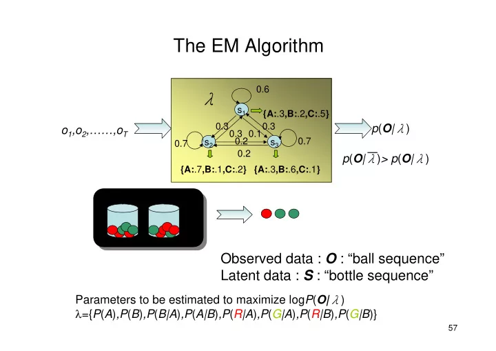
The EM Algorithm 0.6 s 1 {A: .3 ,B: .2 ,C: .5 } 0.30.3 0.20.10.3 - - PowerPoint PPT Presentation

SLIDE 1

57

The EM Algorithm

A B

Observed data : O : “ball sequence” Latent data : S : “bottle sequence”

Parameters to be estimated to maximize logP(O|λ) λ={P(A),P(B),P(B|A),P(A|B),P(R|A),P(G|A),P(R|B),P(G|B)}

• 1,o2,……,oT

p(O|λ)

λ

s2 s1 s3 {A:.3,B:.2,C:.5} {A:.7,B:.1,C:.2} {A:.3,B:.6,C:.1} 0.7 0.30.3 0.2 0.20.10.3 0.7

p(O|λ)> p(O|λ)

0.6

SLIDE 2

58

The EM Algorithm

• Introduction of EM (Expectation Maximization):

– Why EM?

• Simple optimization algorithms for likelihood function

relies on the intermediate variables, called latent (隱藏的)data In our case here, the state sequence is the latent data

• Direct access to the data necessary to estimate the

parameters is impossible or difficult In our case here, it is almost impossible to estimate {A,B, π} without consideration of the state sequence

– Two Major Steps :

• E : expectation with respect to the latent data using the current

estimate of the parameters and conditioned on the

• bservations
• M: provides a new estimation of the parameters according to

Maximum likelihood (ML) or Maximum A Posterior (MAP) Criteria

[ ]

O λ S ,

• E

SLIDE 3

59

The EM Algorithm

• Estimation principle based on observations:

– The Maximum Likelihood (ML) Principle find the model parameter so that the likelihood is maximum for example, if is the parameters of a multivariate normal distribution, and X is i.i.d. (independent, identically distributed), then the ML estimate of is – The Maximum A Posteriori (MAP) Principle find the model parameter so that the likelihood is maximum

( )( )

∑ ∑

= =

− − = =

n i t ML i ML i ML n i i ML

n n

1 1

1 , 1 µ x µ x Σ x µ

{ }

n 2 1

X ,..., X , X = X

( )

n

x x x x ,..., ,

2 1

=

( )

Φ x p Φ Φ

( )

x Φ p

{ }

Σ µ Φ , =

{ }

Σ µ Φ , =

ML and MAP

SLIDE 4

60

The EM Algorithm

• The EM Algorithm is important to HMMs and other

learning techniques

– Discover new model parameters to maximize the log-likelihood

• f incomplete data

by iteratively maximizing the expectation of log-likelihood from complete data

• Using scalar random variables to introduce the EM

algorithm

– The observable training data

• We want to maximize , is a parameter vector

– The hidden (unobservable) data

• E.g. the component densities of observable data , or the

underlying state sequence in HMMs

O S λ

( )

λ O P

( )

λ S O , log P

( )

λ O P log

O

SLIDE 5

61

The EM Algorithm

– Assume we have and estimate the probability that each

• ccurred in the generation of

– Pretend we had in fact observed a complete data pair with frequency proportional to the probability , to computed a new , the maximum likelihood estimate of – Does the process converge? – Algorithm

• Log-likelihood expression and expectation taken over S

( ) ( ) ( )

λ O λ O S λ S O P P P , , =

( ) ( ) ( )

λ O S λ S O λ O , log , log log P P P − =

λ

( )

λ S O , P

λ

O

λ

( )

S O,

S

Bayes’ rule take expectation over S incomplete data likelihood

( )

( )

( ) [ ]

( )

( ) [ ]

( )

( ) [ ]

∑ ∑ ∑

− = =

S S

λ O S λ O S λ S O λ O S λ O λ O S λ O , log , , log , log , log P P P P P P P

s

unknown model setting complete data likelihood

SLIDE 6

62

The EM Algorithm

– Algorithm (Cont.)

• We can thus express as follows
• We want

( )

( )

( ) [ ]

( )

( ) [ ]

( ) ( ) ( ) ( )

( ) [ ]

( ) ( )

( ) [ ]

∑ ∑ ∑ ∑

= = − = − =

S S S S

λ O S λ O S λ λ λ S O λ O S λ λ λ λ λ λ λ O S λ O S λ S O λ O S λ O , log , , , log , , where , , , log , , log , log P P H P P Q H Q P P P P P

( )

( ) ( ) ( )

[ ]

( ) ( ) [ ]

( )

( )

( )

( )

λ λ λ λ λ λ λ λ λ λ λ λ λ λ λ λ λ O λ O , , , , , , , , log log H H Q Q H Q H Q P P + − − = − − − = −

( )

λ O P log

( )

( )

λ O λ O P P log log ≥

SLIDE 7

63

The EM Algorithm

• has the following property

– Therefore, for maximizing , we only need to maximize the Q-function (auxiliary function)

( )

( )

( )

( )

( ) ( )

( )

( ) ( )

( ) [ ]

( )

( )

, , , , ) 1 log ( , , 1 , , , log , , , ≥ + − ∴ = − = − ≤ ⎥ ⎥ ⎦ ⎤ ⎢ ⎢ ⎣ ⎡ ⎟ ⎟ ⎠ ⎞ ⎜ ⎜ ⎝ ⎛ − ≥ ⎥ ⎥ ⎦ ⎤ ⎢ ⎢ ⎣ ⎡ − = + −

∑ ∑ ∑

λ λ λ λ λ O S λ O S λ O S λ O S λ O S λ O S λ O S λ O S λ λ λ λ

S S S

H H P P x x P P P P P P H H Q

( ) ( )

( ) [ ]

∑

=

S

λ S O λ O S λ λ , log , , P P Q

( )

( )

λ λ λ λ , H , H + −

( )

λ O P log

Jensen’s inequality Kullbuack-Leibler (KL) distance

Expectation of the complete data log likelihood with respect to the latent state sequences

SLIDE 8

64

EM Applied to Discrete HMM Training

• Apply EM algorithm to iteratively refine the HMM

parameter vector

– By maximizing the auxiliary function – Where and can be expressed as

) , , ( π B A λ =

( )

( )

( )

[ ]

( ) ( )

( )

∑ ∑

⎥ ⎥ ⎦ ⎤ ⎢ ⎢ ⎣ ⎡ = =

S S

λ S O λ O λ S O λ S O λ O S λ λ , P log P , P , P log , P , Q

( )

( )

( )

( )

( )

( )

∑ ∑ ∑ ∑ ∏ ∏

= − = = − = = − =

+ + = + + = ⎥ ⎦ ⎤ ⎢ ⎣ ⎡ ⎥ ⎦ ⎤ ⎢ ⎣ ⎡ =

+ + +

T t t s T t s s s T t t s T t s s s T t t s T t s s s

t t t t t t t t t

b a P b a P b a P

1 1 1 1 1 1 1 1 1

log log log , log log log log , log ,

1 1 1 1 1 1

• λ

S O

• λ

S O

• λ

S O π π π

( )

λ S O , P

( )

λ S O , P

SLIDE 9

65

EM Applied to Discrete HMM Training

• Rewrite the auxiliary function as

( )

( ) ( )

( )

( )

( ) ( ) ( ) ( )

( )

( ) ( ) ( ) ( ) ( ) ( ) ( )

( )

( ) ( )

( )

∑ ∑ ∑ ∑ ∑ ∑ ∑ ∑ ∑ ∑ ∑ ∑

= = ∈ = = = − = + − = =

⎥ ⎥ ⎦ ⎤ ⎢ ⎢ ⎣ ⎡ = = ⎥ ⎥ ⎦ ⎤ ⎢ ⎢ ⎣ ⎡ = ⎥ ⎥ ⎦ ⎤ ⎢ ⎢ ⎣ ⎡ = = = ⎥ ⎥ ⎦ ⎤ ⎢ ⎢ ⎣ ⎡ = ⎥ ⎥ ⎦ ⎤ ⎢ ⎢ ⎣ ⎡ = = ⎥ ⎥ ⎦ ⎤ ⎢ ⎢ ⎣ ⎡ = + + =

+

N j k v

• t

j t T t s N i N j T t ij t t T t s s N i i s

k t t t t

k b P j ,s P k b P , P Q a P j s i ,s P a P , P Q P i ,s P P , P Q Q Q Q Q

1 all 1 1 1 1 1 1 all 1 1 1 1 all

log log , log , log , log log , , , , ,

1 1

λ O λ O λ O λ S O b λ λ O λ O λ O λ S O a λ λ O λ O λ O λ S O λ b λ a λ λ λ λ

S b S a S π b a π

π π π π

wi yi

? ? ?

SLIDE 10

66

EM Applied to Discrete HMM Training

• The auxiliary function contains three independent

terms, , and

– Can be maximized individually – All of the same form

ij

a

( )

k b j

i

π

( ) ( ) ( )

: when value maximum has and where

∑ ∑ ∑

= = =

= ≥ = = =

N 1 j j j j j N 1 j j N 1 j j j N 2 1

w w y F y , 1 y , y log w y , ,..., y , y g F y y

SLIDE 11

67

EM Applied to Discrete HMM Training

• Proof: Apply Lagrange Multiplier

( )

∑ ∑ ∑ ∑ ∑ ∑ ∑

= = = = = = =

= ∴ − = ⇒ − = ∀ − = ⇒ = + = − + = =

N 1 j j j j N 1 j j N 1 j j N 1 j j j j j j j N 1 j N 1 j j j j N 1 j j j

w w y w w y j y w y w y F 1 y y log w y log w F l l l l l l that Suppose Multiplier Lagrange applying By ∂ ∂

Constraint

SLIDE 12

68

EM Applied to Discrete HMM Training

• The new model parameter set can be

expressed as:

( )

B A π λ , , =

( ) ( )

( )

( ) ( )

( ) ( ) ( )

( ) ( )

( ) ( )

∑ ∑ ∑ ∑ ∑ ∑ ∑ ∑

= = = = = = − = − = − = − = +

= = = = = = = = = = = =

T t t T v

• t

t T t t T v

• t

t i T t t T t t T t t T t t t ij i

i i i s P i s P k b i j i i s P j s i s P a i P i s P

k t k t

1 s.t. 1 1 s.t. 1 1 1 1 1 1 1 1 1 1 1 1

, , , , , , , γ γ λ λ γ ξ λ λ γ λ λ π O O O O O O

SLIDE 13

69

EM Applied to Continuous HMM Training

• Continuous HMM: the state observation does not come

from a finite set, but from a continuous space

– The difference between the discrete and continuous HMM lies in a different form of state output probability – Discrete HMM requires the quantization procedure to map

• bservation vectors from the continuous space to the discrete

space

• Continuous Mixture HMM

– The state observation distribution of HMM is modeled by multivariate Gaussian mixture density functions (M mixtures)

Distribution for State i ( ) ( )

( )

( )

( ) ( )

∑ ∑ ∑

= − = =

⎟ ⎟ ⎟ ⎠ ⎞ ⎜ ⎜ ⎜ ⎝ ⎛ ⎟ ⎠ ⎞ ⎜ ⎝ ⎛ − − − = = =

M k jk jk t jk jk L jk M k jk jk jk M k jk jk j

c N c b c b

1 1 2 / 1 1 1

2 1 exp 2 1 , ; µ

• Σ

µ

• Σ

Σ µ

• π

∑

=

=

M 1 k jk

1 c wi1 wi2 wi3 N1 N2 N3

SLIDE 14

70

EM Applied to Continuous HMM Training

• Express with respect to each single mixture

component

( )

• j

b

( )

• jk

b

( )

( ) ( )

[ ]

⎭ ⎬ ⎫ ⎩ ⎨ ⎧ ⎭ ⎬ ⎫ ⎩ ⎨ ⎧ = ⎭ ⎬ ⎫ ⎩ ⎨ ⎧ ⎭ ⎬ ⎫ ⎩ ⎨ ⎧ =

∑ ∏ ∑ ∑ ∏ ∏ ∏

= = = = − = = − =

+ +

M k T t t k s k s M k M k T t s s s T t t s T t s s s

T t t t t t t t t t

b c a b a P

1 1 1 1 1 1 1 1 1

... ,

1 2 1 1 1 1

• λ

S O π π

( )

( )

[ ]

sequence state with the along sequence component mixture possible the

• f
• ne

: , ,

1 1 1

1 1

S K

• λ

K S O ⎭ ⎬ ⎫ ⎩ ⎨ ⎧ ⎭ ⎬ ⎫ ⎩ ⎨ ⎧ =

∏ ∏

= − =

+

T t t k s k s T t s s s

t t t t t t

b c a P π

( ) ( )

∑ ∑

=

S K

λ K S O λ O , , P P

( )

( )( ) ( )

∑ ∑ ∑ ∏ ∏ ∑

= = = = = =

= + + + + + + + + + =

M k M k M k T t tk TM T T M M T t M k tk

T t t t

a a a a a a a a a a a

1 1 1 1 2 1 2 22 21 1 12 11 1 1

1 2 ...

... ... ... ... : Note

SLIDE 15

71

EM Applied to Continuous HMM Training

• Therefore, an auxiliary function for the EM algorithm can

be written as:

( ) ( )

( )

[ ]

( ) ( )

( )

∑ ∑ ∑ ∑

⎥ ⎥ ⎦ ⎤ ⎢ ⎢ ⎣ ⎡ = =

S K S K

λ K S O λ O λ K S O λ K S O λ O K S λ λ , , log , , , , log , , , P P P P P Q

( )

( )

∑ ∑ ∑

= = − =

+ + + =

+

T t T t k s t k s T t s s s

t t t t t t

c b a P

1 1 1 1

log log log log , , log

1 1

• λ

K S O π

( )

( ) ( )

( )

( )

c , Q , Q , Q , Q , Q

c λ

b λ a λ λ λ λ

b a π

+ + + = π

mixture components Gaussian density functions state transition probabilities initial probabilities

SLIDE 16

72

EM Applied to Continuous HMM Training

• The only difference we have when compared with

Discrete HMM training

( )

( )

( ) ( )

( )

( )

∑ ∑ ∑ ∑ ∑ ∑

= = = = = =

⎪ ⎭ ⎪ ⎬ ⎫ ⎪ ⎩ ⎪ ⎨ ⎧ ⎥ ⎦ ⎤ ⎢ ⎣ ⎡ = = = ⎪ ⎭ ⎪ ⎬ ⎫ ⎪ ⎩ ⎪ ⎨ ⎧ ⎥ ⎦ ⎤ ⎢ ⎣ ⎡ = = =

T t t jk N j M k t t c T t t jk N j M k t t

c k k j s P Q b k k j s P Q

1 1 1 1 1 1

log , , , log , , ,

• λ

Ο c λ

• λ

Ο b λ

b

( )

k j

t

, γ

SLIDE 17

73

EM Applied to Continuous HMM Training

( )

( )

( )

( )

( )

( ) ( )

( ) ( )

( ) ( )

( )

( ) ( )

( ) ( ) ( )

( ) { }

( ) [ ] ( )

∑ ∑ ∑ ∑ ∑ ∑ ∑

= = = − = = = − − − − =

⋅ = ⇒ = − ⇒ ∂ ⎪ ⎭ ⎪ ⎬ ⎫ ⎪ ⎩ ⎪ ⎨ ⎧ ⎥ ⎦ ⎤ ⎢ ⎣ ⎡ ∂ = ∂ ∂ − = ∂ ∂ ⎟ ⎠ ⎞ ⎜ ⎝ ⎛ − − − ⋅ + ⋅ − = ⎟ ⎠ ⎞ ⎜ ⎝ ⎛ − − − = = = = =

T t t T t t t jk T t jk t jk t jk T t N j M k t jk t jk jk t jk jk t jk jk t jk t jk t jk t jk jk t jk t jk t jk L jk jk t t jk M k t t t

j,k j,k j,k b j,k Q b L b N b k k j s P j,k

1 1 1 1 1 1 1 1 1 1 1 2 1 2 1

log , log 2 1 log 2 1 2 log 2 log 2 1 exp 2 1 , ; , , Let γ γ γ γ π π γ

• µ

µ

• Σ

µ

• µ

b λ µ

• Σ

µ

• µ
• Σ

µ

• Σ
• µ
• Σ

µ

• Σ

Σ µ

• λ

Ο

b

( )

here symmetric is and ) (

1 −

+ =

jk

Σ d d x C C x Cx x

T T

SLIDE 18

74

EM Applied to Continuous HMM Training

( ) ( )

( ) ( )

( )

( ) ( )( ) ( )( )

[ ]

( ) ( )

( ) ( )

( )

( )

( )( )

[ ]

( ) ( )

( )( )

( ) ( )

( )( )

( ) (

)( )

[ ]

( )

∑ ∑ ∑ ∑ ∑ ∑ ∑ ∑ ∑ ∑

= = − − = = − − − = = − = − − − − = = = − − − − − − − −

− − ⋅ = ⇒ − − = ⇒ − − = ⇒ = ⎭ ⎬ ⎫ ⎩ ⎨ ⎧ − − − ⋅ ⎟ ⎠ ⎞ ⎜ ⎝ ⎛ − ⇒ ∂ ⎪ ⎭ ⎪ ⎬ ⎫ ⎪ ⎩ ⎪ ⎨ ⎧ ⎥ ⎦ ⎤ ⎢ ⎣ ⎡ ∂ = ∂ ∂ − − − ⋅ − = ⎥ ⎦ ⎤ ⎢ ⎣ ⎡ ⎟ ⎠ ⎞ ⎜ ⎝ ⎛ − − − ⋅ ⋅ ⋅ − = ∂ ∂ ⎟ ⎠ ⎞ ⎜ ⎝ ⎛ − − − ⋅ − ⋅ − =

T t t T t t jk t jk t t jk jk jk t jk t jk t jk jk T t T t t jk jk jk t jk t jk t jk t jk T t T t t jk t T t jk t jk t jk t jk jk t jk T t N j M k t jk t jk jk t jk t jk t jk jk jk t jk t jk t jk jk jk jk jk t jk jk t jk t jk t jk t jk

j,k j,k j,k j,k j,k j,k j,k b j,k Q b L b

1 1 1 1 1 1 1 1 1 1 1 1 1 1 1 1 1 1 1 1 1 1 1 1 1 1 1 1

2 1 log , 2 1 2 1 2 1 log 2 1 log 2 1 2 log 2 log γ γ γ γ γ γ γ γ π µ

• µ
• Σ

Σ Σ µ

• µ
• Σ

Σ Σ Σ Σ Σ µ

• µ
• Σ

Σ Σ µ

• µ
• Σ

Σ Σ

• Σ

b λ Σ µ

• µ
• Σ

Σ Σ µ

• µ
• Σ

Σ Σ Σ Σ

• µ
• Σ

µ

• Σ
• b

T T

d d X ab X X b X a

T T

− =

− )

(

1

( ) [ ]

here symmetric is and ) det( det

jk

Σ d d

T

X X X X

−

⋅ =

SLIDE 19

75

EM Applied to Continuous HMM Training

• The new model parameter set for each mixture

component and mixture weight can be expressed as:

( ) ( ) ( ) ( )

( ) [ ] ( )

∑ ∑ ∑ ∑

= = = =

= = = ⎥ ⎦ ⎤ ⎢ ⎣ ⎡ = = =

T 1 t t T 1 t t t T 1 t t t T 1 t t t t jk

k , j k , j P k k , j s , P P k k , j s , P γ γ

• λ

O λ O

• λ

O λ O µ

( ) ( ) ( )( ) ( ) ( )

( )(

)( )

[ ]

( )

∑ ∑ ∑ ∑

= = = =

− − = = = ⎥ ⎦ ⎤ ⎢ ⎣ ⎡ − − = = =

T 1 t t T 1 t t jk t jk t t T 1 t t t T 1 t t jk t jk t t t jk

k , j k , j P k k , j s , P P k k , j s , P γ γ µ

• µ
• λ

O λ O µ

• µ
• λ

O λ O Σ

( ) ( )

∑ ∑ ∑

= = =

=

T 1 t M 1 k t T 1 t t jk

k , j k , j c γ γ