The Comprehensive Test Ban Treaty (CTBT) The CTBT bans all nuclear - - PowerPoint PPT Presentation

The Comprehensive Test Ban Treaty (CTBT)

The CTBT bans all nuclear explosions for military

• r civilian purposes to limit the proliferation of nu-

clear weapons by cutting a vital link, testing, in their development. A network of seismological, hydroacoustic, infra- sound, and radionuclide sensors will monitor com-

• pliance. Once the Treaty enters into force, on-site

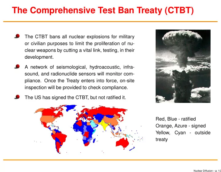
inspection will be provided to check compliance. The US has signed the CTBT, but not ratified it. Red, Blue - ratified Orange, Azure - signed Yellow, Cyan - outside treaty

Nuclear Diffusion – p. 1/2

Can an Opponent Cheat on the CTBT?

U.S. and Russian experiments have demonstrated that seismic signals can be muffled,

• r decoupled, for a nuclear explosion detonated in a large underground cavity.

Such technical scenarios are credible only for yields of at most a few kilotons. Seismic component of the International Monitoring System (INS) for the CTBT is to consist of 170 seismic stations. The INS is expected to detect all seismic events of about magnitude 4 or larger corresponds to an ex- plosive yield of approximately 1 kiloton (the explo- sive yield of 1,000 tons of TNT).

What can be learned from low-yield, sur- reptitious blasts? Can it extrapolated to full-up tests? Demonstration of size of cavity needed to decou- ple a 5 kT blast.

Nuclear Diffusion – p. 2/2

Nuclear Weapons 101

Fissile materials (235U, 233U, 239Pu) are used to make weapons of devastating power. As each nucleus fissions, it emits 2 or so neutrons plus lots of energy. Usually most of the neutrons leave without striking any other nuclei.

235U + n → 236 U∗ →140 Xe + 94Sr + 2n +

≈ 200 MeV Increasing the density creates a ‘chain reaction’ where the emitted neutrons cause

• ther fissions in a self-propagating process.

Only about 8 kg of plutonium or 25 kg of highly-enriched uranium (HEU) is needed is needed to produce a weapon.

U nuclei

235

neutrons A Chain Reaction

Nuclear Diffusion – p. 3/2

HEU Gun-Type Design

The figure to the right shows the ‘Little Boy’ de- sign of the nuclear bomb dropped on Hiroshima. The fissile, 235U is shown in red. A cordite charge was detonated behind one of the pieces of 235U accelerating it to a speed of 300 m/s before it struck the target to form a critical mass (see fig- ure below). A neutron trigger/initiator was used to start the chain reaction.

Nuclear Diffusion – p. 4/2

Critical Mass

In the greatest gathering of scientific talent in human history, the Manhattan Project had the goal ‘to produce a practi- cal military weapon in the form of a bomb in which the energy is released by a fast neutron chain reaction’. This chain re- action will occur when the neutron num- ber density n( r, t) grows exponentially in

• time. Under what conditions will this oc-

cur given the fissile material 235U has a neutron diffusion constant D = 105 m2/s and a neutron creation rate C = 108 s−1? Treat the system as a one-dimensional one of length L in the range 0 < x < L. Neutrons that reach the boundaries escape and no longer contribute to the reaction so require that n(x = 0, t) = n(x = L, t) = 0.

Nuclear fireball 1 ms after det-

• nation showing rope tricks

(Tumbler Snapper).

Nuclear Diffusion – p. 5/2

The Diffusion Equation - Getting Started

Consider a portion of a distribution of matter in a pipe of area A where the num- ber density n depends on position in the x direction.

An(x)dx dx x AJ (x)

x

A AJ (x+dx)

x

Frick’s Law describes the flow of material through volume Jx = −D∂n ∂x where Jx is the x-component of the flow

• f material (units: particles/m2 − s), n

is the number density of the material, and D is a constant of proportionality (unit:m2/s).

Nuclear Diffusion – p. 6/2

The Diffusion Equation - An Example

Consider the one-dimensional diffusion equation corresponding to particles in a long pipe of length L. ∂n(x, t) ∂t = D∂2n ∂x2 + Cn where n(x, t) is the particle density, D is the self-diffusion coefficient, and C is the creation rate. Restrict the problem to the case where there are no sources of particles (C = 0).

• 1. What is the general solution to this differential equation?
• 2. What restrictions are there on the parameters of the solution?
• 3. Suppose the particle density goes to zero at the ends of the pipe so

n(x = 0, t) = n(x = L, t) = 0. What is the particular solution?

Nuclear Diffusion – p. 7/2

The Diffusion Equation - Discretization

A schematic view of the initial values and boundary conditions.

x=0 x=L t=0 Initial condition (red) Boundary conditions (black) Solution in the interior x t

Nuclear Diffusion – p. 8/2

The Diffusion Equation - Discretization

A schematic view of the initial values and boundary conditions.

x=0 x=L t=0 Initial condition (red) Boundary conditions (black) Solution in the interior x t

Now discretize the initial values and boundary conditions.

x=0 t=0 Boundary conditions (black) Solution in the interior x t Initial condition (red) x=L

Nuclear Diffusion – p. 8/2

The Diffusion Equation - The Couplings - 1

x=0 t=0 x t x=L

Nuclear Diffusion – p. 9/2

The Diffusion Equation - The Couplings - 2

x=0 t=0 x t x=L

Nuclear Diffusion – p. 10/2

The Diffusion Equation - The Couplings - 3

x=0 x=L t=0 x t

Nuclear Diffusion – p. 11/2

Euler’s Relation - 1

Euler’s relation (also known as Euler’s formula) is considered the first bridge between the fields of algebra and geometry, as it relates the exponential function to the trigonometric sine and cosine functions. Euler’s relation states that eix = cos x + i sin x Start by noting that ik =              1 k ≡ 0 i k ≡ 1 −1 k ≡ 2 −i k ≡ 3

Nuclear Diffusion – p. 12/2

Euler’s Relation - 2

Using the Taylor series expansions of ex, sin x and cos x it follows that eix =

∞

• n=0

inxn n! =

∞

• n=0

x4n (4n)! + ix4n+1 (4n + 1)! − x4n+2 (4n + 2)! − ix4n+3 (4n + 3)!

• Because the series expansion above is absolutely convergent for all x, we

can rearrange the terms of the series as eix =

∞

• n=0

(−1)n x2n (2n)! + i

∞

• n=0

(−1)n x2n+1 (2n + 1)! = cos x + i sin x

Nuclear Diffusion – p. 13/2

The Diffusion Equation - The Couplings - 4

Explicit method.

x=0 t=0 x t x=L

Implicit method.

x=0 x t x=L t=0

Nuclear Diffusion – p. 14/2

Sample Code - 1

(* Define diffusion parameters. *) Dn = 0.001; (* self diffusion coefficient in mˆ2/shake *) Ln = 0.1; (* size of the region in meters. *) (* parameters for the algorithm. *) tmax = 10.0; (* maximum time in shakes. *) Nxsteps = 20; (* steps in x. *) Ntsteps = 1000; (* steps in time. *) dx = Ln/Nxsteps; (* stepsize in x (m). *) dt = tmax/Ntsteps; (* stepsize in time. *) (* set up the distribution of particles at t=0 so there is always a spike of the same size in the middle. *) n0 = Table[{x, 0, 0}, {x, 0, Ln, dx}]; n0[[Nxsteps/2 + 1, 3]] = 1/dx ; (* initialize the main array. *) particle = Table[0.0, {i, 1, Nxsteps}, {n, 1, Ntsteps}];

Nuclear Diffusion – p. 15/2

Sample Code - 2

(* put in the initial conditions for t=0. *) Do[particle[[i, 1]] = n0[[i, 3]], {i, 1, Nxsteps}]; (* The boundary condition at x=0. *) Do[particle[[1, n]] = 10.0, {n, 2, Ntsteps}]; (* The boundary condition at x=L. *) Do[particle[[Nxsteps, n]] = 0.6, {n, 2, Ntsteps}]; (* constants for the recursion relation. *) A0 = 1 - (2*dt*Dn)/dxˆ2; B0 = (dt*Dn)/dxˆ2; (* main loop. outer loop over time and inner loop over position. *) Do[ Do[particle[[i, n]] = A0*particle[[i, n - 1]] + B0*particle[[i + 1, n - 1]] + B0*particle[[i - 1, n - 1]], {i, 2, Nxsteps - 1}](* end of inner loop *), {n, 2, Ntsteps}](* end of outer loop *)

Nuclear Diffusion – p. 16/2

Oh-Oh

1.00 0.50 5.00 0.10 10.00 0.05 0.01 5 10 50 100 500 1000 t shakes n m1 Neutron Diffusion, Ln0.13, x0.065 m

Nuclear Diffusion – p. 17/2

Oh-Oh

1.00 0.50 5.00 0.10 10.00 0.05 0.01 5 10 50 100 500 1000 t shakes n m1 Neutron Diffusion, Ln0.13, x0.065 m 1.00 0.50 5.00 0.10 10.00 0.05 0.01 5 10 50 100 500 1000 t shakes n m1 Neutron Diffusion, Ln0.13, x0.065 m

Nuclear Diffusion – p. 17/2

The Code - 1

(* Define diffusion parameters. *) Dn = 0.001; (* self diffusion coefficient in mˆ2/shake *) Cn = 1.0; (* Creation rate in fraction/shake. *) Ln = 0.13; (* size of the region in meters. *) (* parameters for the algorithm. *) tmax = 10.0; (* maximum time in shakes. *) Nxsteps = 40; (* steps in x. *) Ntsteps = 3000; (* steps in time. *) dx = Ln/Nxsteps; (* stepsize in x (m). *) dt = tmax/Ntsteps; (* stepsize in time (shakes). *) (* set up the distribution of neutrons at t=0 so there is always a spike of the same size in the middle. *) n0 = Table[{x, 0, 0}, {x, 0, Ln, dx}]; n0[[IntegerPart[Nxsteps/2], 3]] = 1/dx ; (* some test parameters. *) tsigma = dxˆ2/(2*Dn);

Nuclear Diffusion – p. 18/2

The Code - 2

(* monitor the choice of parameters. *) Print["tsigma=", tsigma, " shakes, dt=", dt, " shakes, L=", Ln, " m"] (* initialize the main array. *) neutron = Table[0.0, {i, 1, Nxsteps}, {n, 1, Ntsteps}]; (* put in the initial conditions for t=0. *) Do[neutron[[i, 1]] = n0[[i, 3]], {i, 1, Nxsteps}]; (* The boundary condition at x=0. *) Do[neutron[[1, n]] = 0.0, {n, 2, Ntsteps}]; (* The boundary condition at x=L. *) Do[neutron[[Nxsteps, n]] = 0.0, {n, 2, Ntsteps}]; (* constants for the recursion relation. *) A0 = 1 - (2*dt*Dn)/dxˆ2 + dt*Cn; B0 = (dt*Dn)/dxˆ2;

Nuclear Diffusion – p. 19/2

The Code - 3

(* main loop. outer loop over time and inner loop over position. *) Do[ Do[neutron[[i, n]] = A0*neutron[[i, n - 1]] + B0*neutron[[i + 1, n - 1]] + B0*neutron[[i - 1, n - 1]], {i, 2, Nxsteps - 1}](* end of inner loop *), {n, 2, Ntsteps}] (* end of outer loop *) (* plotting the results in the middle of the x range. *) xcounter = IntegerPart[Nxsteps/2]; xvalue = dx*xcounter; t1 = Table[{dt*(n - 1), neutron[[xcounter, n]]}, {n, 1, Ntsteps}]; t1a = Table[t1[[n, 2]], {n, 2, Ntsteps}]; p1 = ListLogLogPlot[t1, PlotRange -> {{dt, tmax}, {Automatic, Automatic}}, Frame -> True, FrameLabel -> {"t (shakes)", "n (inverse meters)", StringForm["Neutron Diffusion, Ln=‘‘ m", Ln], ""}, Joined -> True, BaseStyle -> Large, PlotStyle -> Thickness[0.005], LabelStyle -> Directive[Larger], ImageSize -> 7*72]

Nuclear Diffusion – p. 20/2