The City College of New York Department of Mechanical Engineering - PowerPoint PPT Presentation

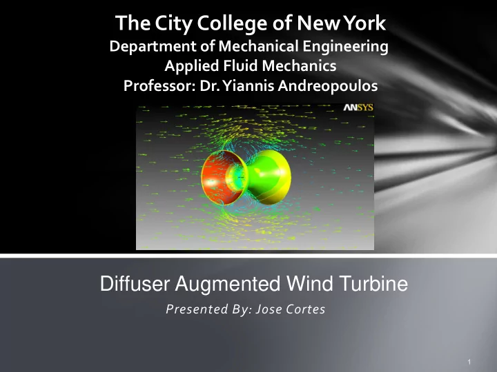
The City College of New York Department of Mechanical Engineering Applied Fluid Mechanics Professor: Dr. Yiannis Andreopoulos Diffuser Augmented Wind Turbine Presented By: Jose Cortes

Abstract Production of electricity using wind turbines is completely clean and renewable. Fossil fuels create emissions that can be harmful to the atmosphere and contribute to global warming; wind power on the other hand provides an environmentally safe alternative. The use and implementation of wind turbines for power production is steadily growing with the demand for clean power generation. With the rising cost of raw materials, initial installation and energy production; customers expect to get the highest power generation per dollar invested. This demand for high efficiency drives us to find ways to quickly improve upon old designs and find alternative methods to maximize the power production.

Goals and Objective In this paper we seek to analyze a diffuser augmented wind turbine using a computational fluid dynamic approach. For our analysis we will be using Ansys-Fluent. The set up for the wind turbine consist of: a converging nozzle which draws the air inside a cylinder increasing the velocity of the incoming air, followed by a short cylinder containing the wind turbine, followed by a diverging nozzle that creates a lower than atmospheric pressure at the outlet helping to draw out the air faster. The result is expected to be an increased in power generated in comparison to a bare wind turbine. In this paper I will investigate the effectiveness of the converging-diverging nozzle adaptation in reference to a bare wind turbine model, and then I will try to improve upon my original design by increasing the inlet size and length at the converging nozzle and comparing the power generated with the other configurations.

Background The blade aerodynamic profile is of outmost importance in for blade performance. Small alterations for the shape of the blade have great impact on the power curve and noise levels. There is a huge selection of aerodynamic profiles that can be selected along with blade shapes and lengths. We can dedicate an indefinite amount of time to the analysis of blade profiles and shapes, but the focus of our study is the impact of the converging-diverging nozzles on the power performance of a wind turbine, and for this reason we will create our own aerodynamic profile and shape for the wind turbine blade. The size of our model is rather small but it will be sufficient to draw conclusions and comparisons.

Profile and Shape

Basic Assumption We will assume a steady, homogenous, irrotational and incompressible laminar flow at the inlet. Static pressure at the upwind and downwind boundaries are equal to atmospheric pressure Governing equations We are going to apply horizontal momentum at the inlet of the cylinder containing the wind turbine and at the outlet. A is the swept area. 𝐺 𝑦 = −𝑈 = 𝑛 𝑊 𝑗𝑜 − 𝑊 𝑝𝑣𝑢 = 𝜍𝐵𝑊 𝑊 𝑗𝑜 − 𝑊 𝑝𝑣𝑢 𝐹𝑟. 1 The thrust at the turbine can also be calculates using the differential pressure between the inlet and outlet multiplied by the swept area A. 𝑈 = 𝑞 𝑗𝑜 − 𝑞 𝑝𝑣𝑢 𝐵 𝐹𝑟. 2 Axial thrust is applied on the wind turbine in the direction of the flow, the turbine applies an equal and opposite direction on the wind. We can apply Bernoulli’s equation to find to find the values of 𝑞 𝑗𝑜 and 𝑞 𝑝𝑣𝑢 𝑞 𝑗𝑜 − 𝑞 𝑝𝑣𝑢 = 1 2 − 𝑊 𝑝𝑣𝑢 2 2 𝜍 𝑊 𝑗𝑜 𝐹𝑟. 3 We can now use equation 3 into equation 2, this yields: 𝑊 = 1 2 𝑊 𝑗𝑜 − 𝑊 𝑝𝑣𝑢 𝐹𝑟. 4 In which V is the stream velocity through the turbine.

Calculation of Wind Power We start by taking by considering the kinetic energy that the air carrying: 𝐿𝐹 = 1 2 𝑛𝑊 2 𝐹𝑟. 5 We are interested in calculating the mass flow rate that is going through the wind turbine. = 𝑊𝑦𝐵𝑦𝜍 = 𝑛 𝑡 𝑛 2 𝑙𝑕 𝑛 3 = 𝑙𝑕 𝑛 𝑡 𝐹𝑟. 6 Where A is again the swept area, V is the average velocity of the air going through the wind turbine, and 𝜍 is the density of the air. The power is calculated by inserting the mass flow rate into Eq. 5, resulting in the following equation: 𝑄 = 1 2 𝐵𝜍𝑊 3 = 𝑥𝑏𝑢𝑢𝑡 This is the ideal power generated by the wind, real life power generation in wind turbines can range from 0.25P to 0.45P.

Solid Modeling The original solid modeling was made with SolidWorks 2011, and it was Imported into the Ansys modeler as a IGS file, later it was remade with the Ansys Design modeler in order to facilitate changes in the geometry.

Ansys Design Modeler Setup Once the solid model was completed, I surrounded it with a cubic enclosure. This enclosure provides a fluid volume which fills the empty spaces that are not occupied by the solid model. The solid model is later suppressed leaving only the fluid enclosure for the analysis.

Solid Model Modification due problems with large blade displacements This modification was implemented after being unsuccessful in getting a solution in the transient model using a dynamic mesh. The problem has to do with the large displacements that occur as the wind turbine rotates. Fluent provides smoothing to deal with small displacements and remeshing to deal with large displacements. Smoothing introduces spring like characteristics to the elements, allowing them to deform as the model undergoes small displacement. Unfortunately for large displacement smoothing does not work well, producing a negative cell error during the program execution. For large displacement remeshing is the adequate choice. Remeshing allows the user to set the largest and smallest element volume as well as the quality of these elements. However due to the large displacements of the blades and the increasing angular speed is very difficult to successfully complete the analysis without encountering a negative volume error.

Solid Model Modification due problems with large blade displacements In order to eliminate negative volume errors, it was necessary to enclose the entire turbine blade inside a cylindrical volume. The purpose is to rotate the volume that encloses the turbine blades and not the turbine blades inside the mesh. The UDF will compute the components of the force hitting the turbine blade faces (which will be set a “wall” type boundary condition) and apply the angular velocity to the cylinder containing the turbine, thus resulting in the same angular velocity.

Solid Model Modification due problems with large blade displacements Rotation Vs. Flow Time (Nozzle Removed Configuration I) 40 Rotation (rad/s) 20 0 0 2 4 6 Time (S)

Mesh Generation

Mesh Generation

Mesh Generation In order to facilitate the selection of the boundary conditions, we will assign names to the different surfaces in the model. Notice the “Cylinder wall inside and outside surfaces”, these were named in order to specify the mesh interaction. The mesh interaction set the parameters to allow the solution to flow through the interface.

Steady State Case The purpose of the steady case in this analysis serves two main goals. First it will allow us to detect any problems with in the meshing, boundary conditions and other settings, and second it will allow us to observe the effect of the converging-diverging nozzle under steady state conditions, which is part of our study. For the steady state condition I will be using my original design, also note that the wind turbine is not rotating, since we have not yet applied the UDF and dynamic mesh settings.

General Settings In the general setting we selected: Type: Pressure Based, Velocity Formulation: Absolute, Time: Steady In the Model window we selected only the laminar model to be on, every other model inclusion is set to be off. We will not be using the energy equation, since we are not dealing with compressible. We need to use the laminar model in order to appreciate the formation of vortices and take into account the losses due to internal friction of the fluid. In the material section we selected the density of air to be constant . This is important to let the program know that the analysis is being performed using a non-compressible fluid.

Boundary conditions Boundary conditions- All Cases Turbine was set to wall (stationary). Box_walls was set to symmetry. Cylinder walls were set to interface. Inlet was set to velocity Inlet with 5m/s x-dir. Interrior-fan_hollow was set to interior. Interior Solid was set to interior. Nozzle was set to wall (stationary). Outlet was set to pressure outlet. The other boundary conditions in the list are set automatically by the interface settings. Symmetry boundary conditions are used when the geometry or the pattern of flow solution possesses mirror symmetry, but it can also be used to model zero-shear slip in viscous walls. Velocity Inlet and pressure outlet are adequate when dealing with incompressible flows.

Boundary conditions Average wind speeds ranges from 5 to 8.5 in most areas per year in the US.

Other Settings

STEADY STATE RESULTS

STEADY STATE RESULTS

STEADY STATE RESULTS

STEADY STATE RESULTS