
SLIDE 1
The Calculus of Computation: Decision Procedures with Applications to Verification by Aaron Bradley Zohar Manna Springer 2007
4- 1
- 4. Induction
4- 2
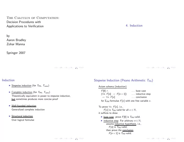
Induction
◮ Stepwise induction (for TPA, Tcons) ◮ Complete induction (for TPA, Tcons)
Theoretically equivalent in power to stepwise induction, but sometimes produces more concise proof
◮ Well-founded induction
Generalized complete induction
◮ Structural induction
Over logical formulae
4- 3
Stepwise Induction (Peano Arithmetic TPA)
Axiom schema (induction) F[0] ∧ . . . base case (∀n. F[n] → F[n + 1]) . . . inductive step → ∀x. F[x] . . . conclusion for ΣPA-formulae F[x] with one free variable x. To prove ∀x. F[x], i.e., F[x] is TPA-valid for all x ∈ N, it suffices to show
◮ base case: prove F[0] is TPA-valid. ◮ inductive step: For arbitrary n ∈ N,
assume inductive hypothesis, i.e., F[n] is TPA-valid, then prove the conclusion F[n + 1] is TPA-valid.
4- 4