The 3-pound universe we live in Cerebrum/Cerebral Cortex Thalamus - PDF document

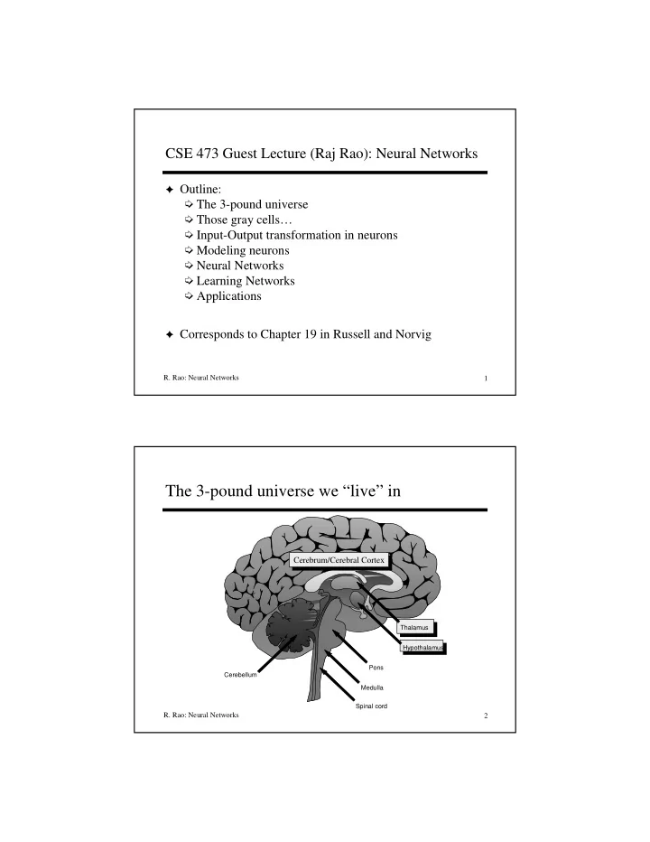
CSE 473 Guest Lecture (Raj Rao): Neural Networks ✦ Outline: ➭ The 3-pound universe ➭ Those gray cells… ➭ Input-Output transformation in neurons ➭ Modeling neurons ➭ Neural Networks ➭ Learning Networks ➭ Applications ✦ Corresponds to Chapter 19 in Russell and Norvig R. Rao: Neural Networks 1 The 3-pound universe we “live” in Cerebrum/Cerebral Cortex Thalamus Hypothalamus Pons Cerebellum Medulla Spinal cord R. Rao: Neural Networks 2

Those gray cells…Neurons From Kandel, Schwartz, Jessel, Principles of Neural Science, 3 rd edn., 1991, pg. 21 R. Rao: Neural Networks 3 Basic Input-Output Transformation in a Neuron Input Spikes Output Spike Spike (= a brief pulse) (Excitatory Post-Synaptic Potential) R. Rao: Neural Networks 4

Communication between neurons: Synapses ✦ Synapses: Connections between neurons ➭ Electrical synapses (gap junctions) ➭ Chemical synapses (use neurotransmitters) ✦ Synapses can be excitatory or inhibitory ✦ Synapses are integral to memory and learning R. Rao: Neural Networks 5 Distribution of synapses on a real neuron… R. Rao: Neural Networks 6

McCulloch–Pitts artificial “neuron” (1943) ✦ Attributes of artificial neuron: ➭ m binary inputs and 1 output (0 or 1) L O ➭ Synaptic weights w ij M P ∑ ( ) = ( ) − + Θ µ ➭ Threshold µ i n t 1 N w n t Q i ij j i j Θ (x) = 1 if x ≥ 0 and 0 if x < 0 Weighted Sum Threshold Inputs Output R. Rao: Neural Networks 7 Properties of Artificial Neural Networks High level abstraction of neural input-output ✦ transformation: Inputs ! weighted sum of inputs ! nonlinear function ! output ✦ Often used where data or functions are uncertain ➭ Goal is to learn from a set of training data ➭ And generalize from learned instances to new unseen data ✦ Key attributes: 1. Massively parallel computation 2. Distributed representation and storage of data (in the synaptic weights and activities of neurons) 3. Learning (networks adapt themselves to solve a problem) 4. Fault tolerance (insensitive to component failures) R. Rao: Neural Networks 8

Topologies of Neural Networks completely connected feedforward recurrent (directed, acyclic) (feedback connections) R. Rao: Neural Networks 9 Networks Types ✦ Feedforward versus recurrent networks ➭ Feedforward: No loops, input ! hidden layers ! output ➭ Recurrent: Use feedback (positive or negative) ✦ Continuous versus spiking ➭ Continuous networks model mean spike rate (firing rate) ✦ Supervised versus unsupervised learning ➭ Supervised networks use a “teacher” ➧ Desired output for each input is provided by user ➭ Unsupervised networks find hidden statistical patterns in input data ➧ Clustering, principal component analysis, etc. R. Rao: Neural Networks 10

Perceptrons ✦ Fancy name for a type of layered feedforward networks = L O M P ∑ ✦ Uses McCulloch-Pitts type neuron: Θ ξ Output M w P N Q i ij j j ✦ Output of neuron is 1 if and only if weighted sum of inputs is greater than 0: Θ (x) = 1 if x ≥ 0 and 0 if x < 0 (a “step” function) Single-layer Multilayer R. Rao: Neural Networks 11 Computational Power of Perceptrons ✦ Consider a single-layer perceptron ➭ Assume threshold units ➭ Assume binary inputs and outputs ∑ ξ = 0 w ij ➭ Weighted sum forms a linear hyperplane j j ✦ Consider a single output network with two inputs ➭ Only functions that are linearly separable can be computed ➭ Example: AND is linearly separable: a AND b = 1 iff a = 1 and b = 1 ξ o = − 1 Linear hyperplane R. Rao: Neural Networks 12

Linear inseparability ✦ Single-layer perceptron with threshold units fails if problem is not linearly separable ➭ Example: XOR ➭ a XOR b = 1 iff (a=0,b=1) or (a=1,b=0) ➭ No single line can separate the “yes” outputs from the “no” outputs! ✦ Minsky and Papert’s book showing such negative results was very influential – essentially killed neural networks research for over a decade! R. Rao: Neural Networks 13 Solution in 1980s: Multilayer perceptrons ✦ Removes many limitations of single-layer networks ➭ Can solve XOR ✦ Two examples of two-layer perceptrons that compute XOR x y ✦ E.g. Right side network ➭ Output is 1 if and only if x + y – 2(x + y – 1.5 > 0) – 0.5 > 0 R. Rao: Neural Networks 14

Multilayer Perceptron The most common activation functions: Output neurons Step function Θ or } Sigmoid function: One or more 1 layers of = 1 g ( a ) − β a + e hidden units (hidden layers) g(a) Ψ (a) g(a) 1 a Input nodes (non-linear “squashing” function) R. Rao: Neural Networks 15 Example: Perceptrons as Constraint Satisfaction Networks out y 2 − 1 1 1 − ? 2 1 2 1 1 2 − 1 − 1 − 1 1 x y x 1 2 R. Rao: Neural Networks 16

Example: Perceptrons as Constraint Satisfaction Networks out 1 =0 y + − < 1 x y 0 2 2 =1 1 + − > 1 x y 0 2 1 1 1 2 − 1 1 x y x 1 2 R. Rao: Neural Networks 17 Example: Perceptrons as Constraint Satisfaction Networks out =0 y 2 =1 1 2 =1 =0 − 1 − 1 1 − − > − − < 2 0 2 0 x y x y x y x 1 2 R. Rao: Neural Networks 18

Example: Perceptrons as Constraint Satisfaction Networks =0 y out 2 =1 − 1 1 1 1 − - − >0 2 1 2 =1 =0 1 x x y 1 2 R. Rao: Neural Networks 19 Perceptrons as Constraint Satisfaction Networks =0 y out 2 =1 1 1 − 1 + − > 1 x y 0 1 2 − 2 1 =1 =0 2 1 1 2 − − < 2 0 x y − 1 − 1 − 1 1 x x y 1 2 R. Rao: Neural Networks 20

Learning networks ✦ We want networks that can adapt themselves ➭ Given input data, minimize errors between network’s output and actual output by changing weights (supervised learning) ➭ Can generalize from learned data to predict new outputs Can this network adapt its weights to solve a problem? How do we train it? R. Rao: Neural Networks 21 Gradient-descent learning (a la Hill-climbing) ✦ Use a differentiable activation function ➭ Try a continuous function f ( ) instead of step function Θ ( ) ➧ First guess: Use a linear unit ➭ Define an error function (cost function or “energy” function) L O 2 Cost function measures M P ∑ ∑ ∑ 1 u = − ξ E M Y w P N Q the network’s squared i ij j 2 i u j errors as a L O M P differentiable function ∂ E ∑ ∑ u Then ∆ w =− η = η M − ξ P ξ Y w N Q ij i ij j j of the weights ∂ w ij u j ✦ Changes weights in the direction of smaller errors ➭ Minimizes the mean-squared error over input patterns µ ➭ Called Delta rule = Widrow-Hoff rule = LMS rule R. Rao: Neural Networks 22

Learning via Backpropagation of Errors ✦ Backpropagation is just gradient-descent learning for multilayer feedforward networks ✦ Use a nonlinear , differentiable activation function ➭ Such as a sigmoid: ≡ ∑ 1 a f ≡ + ξ f where h w ij j − η 1 exp 2 h j ✦ Result: Can propagate credit/blame back to internal nodes ➭ Change in weights for output layer is similar to Delta rule ➭ Chain rule (calculus) gives ∆ w ij for internal “hidden” nodes R. Rao: Neural Networks 23 Backpropagation V j R. Rao: Neural Networks 24

Backpropagation (for Math lovers’ eyes only!) ✦ Let A i be the activation (weighted sum of inputs) of neuron i ✦ Let V j = g(A j ) be output of hidden unit j ✦ Learning rule for hidden-output connection weights: ➭ ∆ W ij = - η∂Ε/∂ W ij = η Σ µ [d i – a i ] g ’ (A i ) V j = η Σ µ δ i V j ✦ Learning rule for input-hidden connection weights: ➭ ∆ w jk = - η ∂Ε/∂ w jk = - η ( ∂Ε/∂ V j ) ( ∂ V j /∂ w jk ) { chain rule } =η Σ µ,ι ( [d i – a i ] g ’ (A i ) W ij ) ( g ’ (A j ) ξ k ) = η Σ µ δ j ξ k R. Rao: Neural Networks 25 Hopfield networks (example of recurrent nets) ✦ Act as “autoassociative” memories to store patterns ➭ McCulloch-Pitts neurons with outputs -1 or 1, and threshold Θ ➭ All neurons connected to each other ➧ Symmetric weights (w ij = w ji ) and w ii = 0 ➭ Asynchronous updating of outputs ➧ Let s i be the state of unit i ➧ At each time step, pick a random unit ➧ Set s i to 1 if Σ j w ij s j ≥ µ i ; otherwise, set s i to -1 completely connected R. Rao: Neural Networks 26

Hopfield networks ✦ Network converges to cost function’s local minima which store different patterns x 1 x 4 ✦ Store p N-dimensional pattern vectors x 1 , …, x p using a “Hebbian” learning rule: ➭ w ji = 1/N Σ m=1,..,p x m,j x m,i for all j ≠ i; 0 for j = i ➭ W = 1/N Σ m=1,..,p x m x mT (outer product of vectors; diagonal zero) ➧ T denotes vector transpose R. Rao: Neural Networks 27 Pattern Completion in a Hopfield Network ! Network converges Local minimum from here (“attractor”) of cost to here (or “energy”) function stores pattern R. Rao: Neural Networks 28