Neural Networks Find a way to teach networks to do a certain - - PowerPoint PPT Presentation

Neural Networks

Mark van Rossum

School of Informatics, University of Edinburgh

January 15, 2018

1 / 28

Goals: Understand how (recurrent) networks behave Find a way to teach networks to do a certain computation (e.g. ICA) Network choices Neuron models: spiking, binary, rate (and its in-out relation). Use separate inhibitory neurons (Dale’s law)? Synaptic transmission dynamics?

2 / 28

Overview

Feedforward networks

Perceptron Multi-layer perceptron Liquid state machines Deep layered networks

Recurrent networks

Hopfield networks Boltzmann Machines

3 / 28

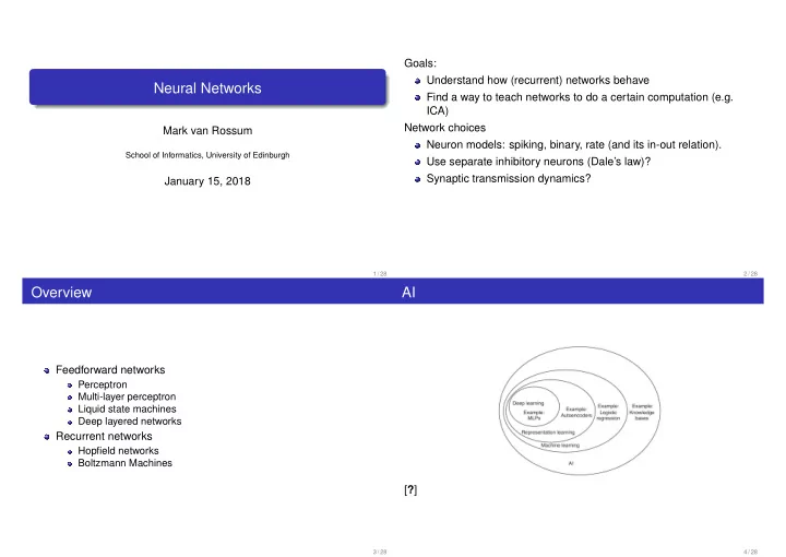
AI

[?]

4 / 28

AI

[?]

5 / 28

History

McCullough & Pitts (1943): Binary neurons can implement any finite state machine. Rosenblatt: Perceptron learning rule: Learning of (some) classification problems. Backprop: Universal function approximator. Generalizes, but has local maxima.

6 / 28

Perceptrons

Supervised binary classification of N-dimensional x pattern vectors. y = H(w.x + b), H is step function General trick: replace bias b = wb.1 with ’always on’ input. Perceptron learning algorithm: Learnable if patterns are linearly seperable. If learnable, rule converges. XXXCOntinuous input??? XXX figure Cerebellum?

7 / 28

Multi-layer perceptron (MLP)

Overcomes limited functions the single perceptron With continuous units, MLP can approximate any function! Tradionally one hidden layer. More layers does enhance repetoire (but could help learning, see below). Learning: backpropagation of errors. Error: E = Eµ = P

µ=1(yµ goal − yµ actual(xµ; w))2 Gradient descent

(batch) ∆wij = −η ∂E

∂wij , where w are all the weights (input →

hidden, hidden → output, bias).

• ther cost functions are possible

XXX picture Stochastic descent: use ∆wij = − ∂Eµ

∂wij .

Learning MLPs is slow, local maxima.

8 / 28

Deep MLPs

Traditional MLPs are also called shallow While deeper nets do not have more computational power, they can lead to better representations. Better representations lead to better generalization and better learning. Learning slows down in deep networks, as transfer functions g() saturate at 0 or 1. Solutions:

pre-training convolutional networks

Better representation by adding noisy/partial stimuli

9 / 28

Liquid state machines

[?] Motivation: arbitrary spatio-temporal computation without precise design. Create pool of spiking neurons with random connections. Results in very complex dynamics if weights are strong enough Similar to echo state networks (but those are rate based). Both are known as reservoir computing Similar theme as HMAX model: only learn at the output layer.

10 / 28 11 / 28

Optimal reservoir?

Best reservoir has rich yet predictable dynamics. Edge of Chaos [?] Network 250 binary nodes, wij = N(0, σ2) (x-axis is recurrent strength)

12 / 28

Optimal reservoir?

Task: Parity(in(t), in(t − 1), in(t − 2)) Best (darkest in plot) at edge of chaos. Does chaos exist in the brain? In spiking network models: yes [?] In real brains: ?

13 / 28

Relation to Support Vector Machines

Map problem in to high dimensional space F; there it often becomes linearly separable. This can be done without much computational overhead (kernel trick).

14 / 28

Hopfield networks

All to all connected network (can be relaxed) Binary units si = ±1, or rate with sigmodial transfer. Dynamics si(t + 1) = sign(

j wijsj(t))

Using symmetric weights wij = wji, we can define energy E = − 1

2

• ij siwijsj.

15 / 28

Under these conditions network moves from initial condition (stimulus, s(t = 0) = x) into the closest attractor state (’memory’). Auto-associative, pattern completion Simple (suboptimal) learning rule: wij = M

µ xµ i xµ j

(µ indexes patterns xµ).

16 / 28

Indirect experimental evidence using maze deformation[?]

17 / 28

Winnerless competition

How to escape from attractor states? Noise, asymmetric connections, adaptation. From [?].

18 / 28

Boltzmann machines

Hopfield network is not ’smart’. In Hopfield network it is impossible to learn only (1, 1, −1), (−1, −1, −1), (1, −1, 1), (−1, 1, 1) but not (−1, −1, 1), (1, 1, 1), (−1, 1, −1), (1, −1, 1) (XOR again)... Because xi =

• xixj
• = 0

Two, somewhat unrelated, modifications: Introduce hidden units, these can extract features. Stochastic updating: p(si = 1) =

1 1+e−βEi

Ei =

j wijsj − θi, E = i Ei.

T = 1/β is temperature (set to some arbitrary value).

19 / 28

Learning in Boltzmann machines

The generated probability for state sα, after equilibrium is reached, is given by the Boltzmann distribution Pα = 1 Z

• γ

e−βHαγ Hαγ = −1 2

• ij

wijsisj Z =

• αβ

e−βHαγ where α labels states of visible units, γ the hidden states.

20 / 28

As in other generative models, we match true distribution to generated

• ne.

Minimize KL divergence between input and generated dist. C =

• α

Gα log Gα Pα Minimize to get [?] ∆wij = ηβ[

• sisj
• clamped −
• sisj
• free]

(note, wij = wji) Wake (’clamped’) phase vs. sleep (’dreaming’) phase Clamped phase: Hebbian type learning. Average over input patterns and hidden states. Sleep phase: unlearn erroneous correlations. The hidden units will ’discover’ statistical regularities.

21 / 28

Boltzmann machines: applications

Shifter circuit. Learning symmetry [?]. Create a network that categorizes horizontal, vertical, diagonal symmetry (2nd order predicate).

22 / 28

Restricted Boltzmann

Need for multiple relaxation runs for every weight update (triple loop), makes training Boltzmann networks very slow. Speed up learning in restricted Boltzmann: No hidden-hidden connections Don’t wait for the sleep state to fully settle Stack multiple layers (deep-learning) Application: high quality autoencoder (i.e. compression) [?] [also good webtalks by Hinton on this]

23 / 28

Le etal. ICML 2012 Deep auto-encoder network with 109 weights learns high level features from images unsupervised.

24 / 28

Relation to schema learning?

Maria Shippi & MvR Cortex learns semantic /scheme (i.e. statistical) information Presence of a schema can speed up subsequent fact learning.

25 / 28

Discussion

Networks still very challenging Can we predict activity? What is the network trying to do? What are the learning rules?

26 / 28

References I

27 / 28