SLIDE 1
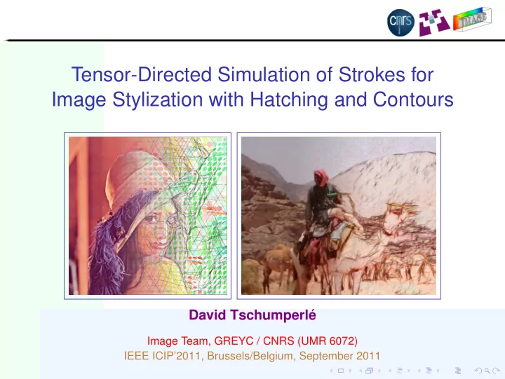
Tensor-Directed Simulation of Strokes for Image Stylization with Hatching and Contours
David Tschumperlé
Image Team, GREYC / CNRS (UMR 6072) IEEE ICIP’2011, Brussels/Belgium, September 2011
SLIDE 2 Context & Motivation
Context : Non-Photorealistic Rendering (NPR). Motivation : Render a photograph as a sketch or a pencil drawing. Method : B&W stroke-based algorithm. Place (black) graphic primitives on an white canvas, according to the geometry of the initial image. Then, colorize the result. − →
Original color image Final rendering
SLIDE 3 Overview : State of the art of B&W NPR
Deussen-Hiller-etal (stipple drawing) Durand-Ostromoukhov-etal (interactive method) Salisbury-Wong-etal (oriented textures) Hertzmann-Zorin (from 3d models) Winkenbach-Salesin (from 3d models) Salisbury-Anderson-etal (interactive method)
SLIDE 4
Contributions of this work
We propose (yet) another stroke-based algorithm with : Straight or curved lines as graphic primitives. 2nd-order tensors for analyzing the local image geometry and modeling the pencil paths. Ability to render image contours and hatching within the same single process. Use the flexibility of the tensor model to allow multiple drawing styles with the same algorithm and from the same input image. = ⇒ Try to simulate pencil strokes as they would be drawn by an artist !
SLIDE 5
Illustration of the proposed method
Same input image leads to multiple styles of pencil rendering
SLIDE 6 A first naive approach
1
Compute the image luminance Y : Ω → R, and its smoothed gradient ∇Yσ = ∇Y ∗ Gσ.
2
Create an empty (white) canvas S : Ω → R.
3
Repeat N times :
1
Pick one random position X = (x, y) in Ω.
2
Draw a semi-transparent straight line X − Lξ(X) → X + Lξ(X) on S, where ξ(X) =
∇Y ⊥
σ(X)
∇Yσ(X) (contour direction at X).
Color image I Luminance Y Smoothed gradient ∇Yσ
SLIDE 7
After 1st iteration
Canvas S
SLIDE 8
After 200th iterations
Canvas S
SLIDE 9
After 600th iterations
Canvas S
SLIDE 10
After 1200th iterations
Canvas S
SLIDE 11
After 4800th iterations
Canvas S
SLIDE 12
After 10000th iterations
Canvas S
SLIDE 13
After 10000th iterations (colorized)
Canvas S + Colorization
SLIDE 14
Edge-focused modification
Draw a pencil stroke at X only when ∇Yσ(X) > ǫ (i.e. X is on a significant edge).
SLIDE 15
Edge-focused modification (colorized)
Draw a pencil stroke at X only when ∇Yσ(X) > ǫ (i.e. X is on a significant edge).
SLIDE 16 Things that are missing
1
Only straight lines.
2
Poor analysis of the image geometry (simple gradient, no analysis
3
No spatial coherence (or no drawing) on flat image regions. = ⇒ Can be easily improved by considering tensor models !
SLIDE 17 From diffusion tensors...
Inspired by the formalism of diffusion tensors, used for directing PDE-based anisotropic smoothing processes.
[Weickert:98,Tschumperle-Deriche:03,...]
∂I ∂t = div (D∇I)
∂I ∂t = trace (DH) Based on the analysis of the local image geometry through the computation of the structure tensor [DiZenzo:86]. Gα,σ = (
∇Iiα ∇IT
iα) ∗ Gσ
Eigenvalues/eigenvectors of Gα,σ are robust local geometric estimators of the image structures. Diffusion tensors D are built upon Gα,σ and direct the smoothing process − → Anisotropic diffusion.
SLIDE 18 From diffusion tensors (illustrated)...
T = λ1 uuT + λ2 vvT = a b b c
Structure tensors field Gσ Diffusion tensors field D
= ⇒ Diffusion tensors model the way a digital painter would apply the “smudge tool” to smooth the noise and remove image artefacts.
SLIDE 19 ...to stroke tensors
Structure tensors are able to locally distinct between different types of image regions :
1
Flat regions : Small isotropic tensors.
2
Contours : Anisotropic tensors, oriented ⊥ to the contour.
3
Small-scale texture : Large isotropic tensors.
From an “sketching” point of view, this would correspond to differents drawing behaviors :
1
Flat regions or textures : Regular strokes forming a coherent hatching pattern.
2
Contours : Oriented strokes, along the contour direction.
= ⇒ Strokes geometry can be successfuly modeled by a tensor field T that depends on G(α,σ) !
[See paper content for more details about our proposal]
SLIDE 20 ...to stroke tensors
From an “sketching” point of view, this would correspond to differents drawing behaviors :
1
Flat regions or textures : Regular strokes forming a coherent hatching pattern.
2
Contours : Oriented strokes, along the contour direction.
− → = ⇒ Stroke tensors variability will lead to different drawing styles.
SLIDE 21 From stroke tensors...
Question : How to draw strokes on canvas S with respect to the stroke tensor field T, such that :
1
Small isotropic tensors locally render very few strokes.
2
Large isotropic tensors locally render hatches.
3
Anisotropic tensors locally render oriented contour strokes.
? − →
SLIDE 22 ...To stroke drawing
Stroke throwing algorithm : Initialize an empty canvas S and compute the stroke tensors T from the input image I. For each angle γ from a given set [γ0, γ1, ..., γN], do :
1
Compute vector field wγ = √ Taγ with aγ = (cos γ sin γ)T.
2
Repeat N times :
1
Pick one random position X = (x, y) in Ω.
2
Draw a semi-transparent straight line X − Lξ(X) → X + Lξ(X) or a streamline of wγ starting from X and of length L, on S.
The stroke tensors are used to distort each direction aγ, according to the geometry of the input image. The choosen number of angles γ set the style of the hatches. Streamlines allow drawn strokes to be curved.
SLIDE 23
Illustration of the algorithm
Input image (synthetic).
SLIDE 24
Illustration of the algorithm
Computed field of stroke tensors.
SLIDE 25
Illustration of the algorithm
Some streamline strokes drawn for γ = 0o.
SLIDE 26
Illustration of the algorithm
Some streamline strokes drawn for γ = 48o.
SLIDE 27
Illustration of the algorithm
Some streamline strokes drawn for γ = 96o.
SLIDE 28
Illustration of the algorithm
Some streamline strokes drawn for γ = 45o and γ = 135o.
SLIDE 29
Illustration of the algorithm
Final result with straight lines, γ = 45o and γ = 135o.
SLIDE 30
Illustration of the algorithm
Final result with curved lines, γ = 45o and γ = 135o.
SLIDE 31
Colorization step
Colorization combines the B&W sketch canvas and the colors of the input image, to add colors to the generated sketch. Here, we tried very simple combinations only, also known as layer blending modes : Soft light, hard light, overlay,.... All results shown afterwards are using these simple coloring techniques.
Input image B&W sketch “Colorized” result
SLIDE 32
Some results
Some straightforward applications of the sketch algorithm, with simple colorization steps...
SLIDE 33
Some results
SLIDE 34
Some results
SLIDE 35
Some results
Can be used to simulate several different drawing steps towards a final painting.
Step 1 (straight strokes)
SLIDE 36
Some results
Step 2 (curved strokes)
SLIDE 37
Some results
Step 3 (curved strokes + colorization)
SLIDE 38
Some results
Step 4 (curved strokes + colorization)
SLIDE 39
Some results
Final painting (the only input image of the algorithm !)
SLIDE 40
Some results
(Colors do not have to match the input image)
SLIDE 41
Advanced results
Several sketch results can be also merged together to render even more complex rendering (courtesy of Tom Keil).
SLIDE 42
Advanced results
Several sketch results can be also merged together to render even more complex rendering (courtesy of Tom Keil).
SLIDE 43
Advanced results
SLIDE 44
Advanced results
SLIDE 45
Advanced results
SLIDE 46
Advanced results
SLIDE 47
Advanced results
SLIDE 48 Conclusions and perspectives
Conclusions : We have proposed a B&W stroke-based algorithm for simulating the drawing of lines, to convert photographs into sketchs.
1
It uses tensor fields to deal with the geometry both of the image and the strokes.
2
It defines a way to draw strokes according to the geometric shape
Perspectives :
1
Find the best ways to model the stroke tensors according to a given artistic style.
2
Improve the colorization step.
3
Model the thickness of strokes.
4
Deal with image sequences (temporal coherence).
SLIDE 49
Do it yourself !
The algorithm code is available in G’MIC, a powerful framework for image processing, developed at the GREYC/Image lab. http://gmic.sourceforge.net Try our sketch algorithm, with the G’MIC plug-in for GIMP.
SLIDE 50
Questions ?
(Don’t shoot the speaker !)