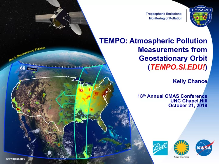
TEMPO: Atmospheric Pollution Measurements from Geostationary Orbit - - PowerPoint PPT Presentation

TEMPO: Atmospheric Pollution Measurements from Geostationary Orbit (TEMPO.SI.EDU!)

Kelly Chance

18th Annual CMAS Conference UNC Chapel Hill October 21, 2019

Hourly a atmo tmospheri eric p c polluti tion from

• m g

geost

• station
• nary E

Earth o

• rbi

bit

PI: Kelly Chance, Smithsonian Astrophysical Observatory Deputy PI: Xiong Liu, Smithsonian Astrophysical Observatory Instrument Development: Ball Aerospace Project Management: NASA LaRC Other Institutions: NASA GSFC, NOAA, EPA, NCAR, Harvard, UC Berkeley, St. Louis U, U Alabama Huntsville, U Nebraska, RT Solutions, Carr Astronautics International collaboration: Mexico, Canada, Cuba, Korea, U.K., ESA, Spain Selected Nov. 2012 as NASA’s first Earth Venture Instrument

• Instrument delivery 2018
• NASA has arranged hosting on a commercial geostationary

communications satellite with launch expected 2/2022 Provides hourly daylight observations to capture rapidly varying emissions & chemistry important for air quality

• Distinguishes boundary layer from free tropospheric & stratospheric
• zone

North American component of an international constellation for air quality observations

10/21/19 2

The view from GEO

10/21/19

The old Chance place 22,236 miles away!

3

Geostationary orbit

• pportunities of interest

10/21/19 4

(typical) Between 90 W and 110 W, there are nine

• wner operators of 30 satellites including
• lder models still used in this location:

Direct TV Group (7) AGS (5) Intelsat (5) Telesat (4) Hughes Network Systems (3) Echostar (2) SkyTerra (2) Inmarsat (1) ICO Global Communications (1)

TEMPO will be located at 91o West

TEMPO status

• Instrument completed, accepted, delivered,

now in storage

• Commercial geostationary satellite host

selected for launch in February 2022 to 91oW

10/21/19 5

Ready for storage

10/21/19 6

TEMPO instrument concept

• Measurement technique
• Imaging grating spectrometer measuring solar backscattered Earth radiance
• Spectral band & resolution: 290-490 + 540-740 nm @ 0.6 nm FWHM, 0.2 nm

sampling

• 2 2-D, 2k×1k, detectors image the full spectral range for each geospatial scene
• Field of Regard (FOR) and duty cycle
• Mexico City/Yucatan, Cuba to the Canadian oil sands, Atlantic to Pacific
• Instrument slit aligned N/S and swept across the FOR in the E/W direction,

producing a radiance map of Greater North America in one hour

• Spatial resolution
• 2.1 km N/S × 4.7 km E/W native pixel resolution (9.8 km2)
• Co-add/cloud clear as needed for specific data products
• Standard data products and sampling rates
• Most sampled hourly, including eXceL O3 (troposphere, PBL)
• NO2, H2CO, C2H2O2, SO2 sampled hourly (average results for ≥ 3/day if needed)
• Measurement requirements met up to 50o for SO2, 70o SZA for other products

10/21/19 7

TEMPO science questions

• 1. What are the temporal and spatial variations of emissions of

gases and aerosols important for air quality and climate?

• 2. What are the physical, chemical, and dynamical processes

that transform tropospheric composition and air quality

• ver scales ranging from urban to continental, diurnally to

seasonally?

• 3. How does air pollution drive climate forcing and how does

climate change affect air quality on a continental scale?

• 4. How can observations from space improve air quality

forecasts and assessments for societal benefit?

• 5. How does intercontinental transport affect air quality?
• 6. How do episodic events, such as wild fires, dust outbreaks,

and volcanic eruptions, affect atmospheric composition and air quality?

10/21/19 8

Team Member Institution Role Responsibility

• K. Chance

SAO PI Overall science development; Level 1b, H2CO, C2H2O2

• X. Liu

SAO Deputy PI Science development, data processing; O3 profile, tropospheric O3

• J. Al-Saadi

LaRC Deputy PS Project science development

• J. Carr

Carr Astronautics Co-I INR Modeling and algorithm

• M. Chin

GSFC Co-I Aerosol science

• R. Cohen

U.C. Berkeley Co-I NO2 validation, atmospheric chemistry modeling, process studies

• D. Edwards

NCAR Co-I VOC science, synergy with carbon monoxide measurements

• J. Fishman
• St. Louis U.

Co-I AQ impact on agriculture and the biosphere

• D. Flittner

LaRC Project Scientist Overall project development; STM; instrument cal./char.

• J. Herman

UMBC Co-I Validation (PANDORA measurements)

• D. Jacob

Harvard Co-I Science requirements, atmospheric modeling, process studies

• S. Janz

GSFC Co-I Instrument calibration and characterization

• J. Joiner

GSFC Co-I Cloud, total O3, TOA shortwave flux research product

• N. Krotkov

GSFC Co-I NO2, SO2, UVB

• M. Newchurch
• U. Alabama Huntsville

Co-I Validation (O3 sondes, O3 lidar) R.B. Pierce NOAA/NESDIS Co-I AQ modeling, data assimilation

• R. Spurr

RT Solutions, Inc. Co-I Radiative transfer modeling for algorithm development

• R. Suleiman

SAO Co-I, Data Mgr. Managing science data processing, BrO, H2O, and L3 products

• J. Szykman

EPA Co-I AIRNow AQI development, validation (PANDORA measurements)

• O. Torres

GSFC Co-I UV aerosol product, AI

• J. Wang
• U. Iowa

Co-I Synergy w/GOES-R ABI, aerosol research products

• J. Leitch

Ball Aerospace Collaborator Aircraft validation, instrument calibration and characterization

• D. Neil

LaRC Collaborator GEO-CAPE mission design team member

TEMPO Science Team, U.S.

10/21/19 9

Team Member Institution Role Responsibility Randall Martin Dalhousie U. Collaborator Atmospheric modeling, air mass factors, AQI development Chris McLinden Environment Canada Collaborator Canadian air quality coordination Michel Grutter de la Mora UNAM, Mexico Collaborator Mexican air quality coordination Gabriel Vazquez UNAM, Mexico Collaborator Mexican air quality, algorithm physics Amparo Martinez INECC, Mexico Collaborator Mexican environmental pollution and health

• J. Victor Hugo Paramo Figeuroa

INECC, Mexico Collaborator Mexican environmental pollution and health Brian Kerridge Rutherford Appleton Laboratory, UK Collaborator Ozone profiling studies, algorithm development Paul Palmer Edinburgh U., UK Collaborator Atmospheric modeling, process studies Alfonso Saiz-Lopez CSIC, Spain Collaborator Atmospheric modeling, process studies Juan Carlos Antuña Marrero GOAC, Cuba Collaborator Cuban Science team lead, Cuban air quality Osvaldo Cuesta GOAC, Cuba Collaborator TEMPO validation, Cuban air quality René Estevan Arredondo GOAC, Cuba Collaborator TEMPO validation, Cuban air quality

• J. Kim

Yonsei U. Collaborators, Science Advisory Panel Korean GEMS, CEOS constellation of GEO pollution monitoring C.T. McElroy York U. Canada CSA PHEOS, CEOS constellation of GEO pollution monitoring

• B. Veihelmann

ESA ESA Sentinel-4, CEOS constellation of GEO pollution monitoring J.P. Veefkind KNMI ESA Sentinel-5P (TROPOMI)

TEMPO Science Team, non-U.S.

10/21/19 10

Air quality requirements from the GEO- CAPE Science Traceability Matrix

10/21/19 11

Ultraviolet/ visible species (GOME, SCIA, OMI, OMPS, TEMPO, etc.)

10/21/19 12

Typical TEMPO-range spectra (from ESA GOME-1)

10/21/19 13

Low Earth orbit: Sun-synchronous nadir heritage

10/21/19 14

Instrument Detectors Spectral Coverage [nm] Spectral Res. [nm] Ground Pixel Size [km2] Global Coverage

GOME-1 (1995-2011) Linear Arrays 240-790 0.2-0.4 40×320 (40×80 zoom) 3 days SCIAMACHY (2002-2012) Linear Arrays 240-2380 0.2-1.5 30×30/60/90 30×120/240 6 days OMI (2004) 2-D CCD 270-500 0.42-0.63 13×24 - 42×162 daily GOME-2a,b (2006, 2012) Linear Arrays 240-790 0.24-0.53 40×80 (40×10 zoom) near-daily OMPS-1 (2011) 2-D CCDs 250-380 0.42-1.0 50×50 daily

Previous experience (since 1985 at SAO and MPI)

Scientific and operational measurements of pollutants O3, NO2, SO2, H2CO, C2H2O2 (& CO, CH4, BrO, OClO, ClO, IO, H2O, O2-O2, Raman, aerosol, ….)

LEO measurement capability

10/21/19 15

A full, minimally-redundant, set of polluting gases, plus aerosols and clouds is now measured to very high precision from

• satellites. Ultraviolet and visible spectroscopy
• f backscattered radiation provides O3

(including profiles and tropospheric O3), NO2 (for NOx), H2CO and C2H2O2 (for VOCs), SO2, H2O, O2, O2-O2, N2 and O2 Raman scattering, and halogen oxides (BrO, ClO, IO, OClO). Satellite spectrometers we planned since 1985 began making these measurements in 1995.

Kilauea activity, source of the VOG event in Honolulu

• n 9 November 2004

GOME, SCIAMACHY, and OMI examples

NO2 O3

strat trop

SO2 C2H2O2 H2CO H2O

Baseline and threshold data products

Species/Products Required Precision Temporal Revisit

0-2 km O3 (Selected Scenes) Baseline only 10 ppbv 2 hour Tropospheric O3 10 ppbv 1 hour Total O3 3% 1 hour Tropospheric NO2 1.0 × 1015 molecules cm-2 1 hour Tropospheric H2CO 1.0 × 1016 molecules cm-2 3 hour Tropospheric SO2 1.0 × 1016 molecules cm-2 3 hour Tropospheric C2H2O2 4.0 × 1014 molecules cm-2 3 hour Aerosol Optical Depth 0.10 1 hour

• Minimal set of products sufficient for constraining air quality
• Across Greater North America (GNA): 18°N to 58°N near 100°W, 67°W to 125°W near

42°N

• Data products at urban-regional spatial scales

– Baseline ≤ 60 km2 at center of Field Of Regard (FOR) – Threshold ≤ 300 km2 at center of FOR

• Temporal scales to resolve diurnal changes in pollutant distributions
• Geolocation uncertainty of less than 4 km
• Mission duration, subject to instrument availability

– Baseline 20 months – Threshold 12 months 10/21/19 17

TE TEMP MPO O ho hourly NO y NO2 sw sweep (GE GEO @9 O @92.85W)

Boresight: 34N, 91W ~ 2034 good N/S pixels

• ~ 1282 scans/hr
• ~ 2.6 M pixels/hr
• Data rate: ~31.2

Mbs (~20 times of OMI data, comparable to TROPOMI)

• Scanning partial

FOV at ≤ 10 min allowed up to 25%

• f time

10/21/19 18

TE TEMP MPO O footprint (GE GEO O @91º 91º W) W)

Location N/S (km) E/W (km) GSA (km2) VZA (o) Boresight 2.0 4.8 9.5 39.3 36.5oN, 100oW 2.1 4.8 10.1 42.4 Washington, DC 2.3 5.1 11.3 48.0 Seattle 3.2 6.2 16.8 61.7 Los Angeles 2.1 5.6 11.3 48.0 Boston 2.5 5.5 13.0 53.7 Miami 1.8 4.9 8.6 33.2 San Juan 1.7 5.6 9.2 37.4 Mexico City 1.6 4.7 7.7 23.9

• Can. tar sands

4.1 5.6 20.8 67.0 Juneau 6.1 9.1 33.3 75.3

• Boresight at 33.76oN, 92.85oW

10/21/19 19

Los Angeles coverage

10/21/19 20

Global pollution monitoring constellation

Sentinel-5P (once per day) TEMPO (hourly) Sentinel-4 (hourly) GEMS (hourly)

Courtesy Jhoon Kim, Andreas Richter

80-115°W 0° 2021+ launch 128.2°E 2019 launch

10/21/19 21

The TEMPO Green Paper

Chemistry, physics, and meteorology experiments with the Tropospheric Emissions: Monitoring of Pollution instrument

Now at: https://www.cfa.harvard.edu/atmosphere/publications.html

• K. Chancea, X. Liu a, C. Chan Millera, G. González Abad a, G. Huangb, C. Nowlan a, A. Souri a, R. Suleiman a, K. Sunc, H. Wang a, L. Zhu a, P. Zoogman a, J. Al-Saadid, J.-C. Antuña-

Marreroe, J. Carrf, R. Chatfieldg, M. Chinh, R. Coheni, D. Edwardsj, J. Fishmank, D. Flittnerd, J. Geddesl, M. Grutterm, J.R. Hermann, D.J. Jacobo, S. Janzh J. Joinerh, J. Kimp, N.A. Krotkovh, B. Leferq, R.V. Martin,a,r,s, O.L. Mayol-Bracerot, A. Naegeru, M. Newchurchu, G.G. Pfisterj, K. Pickeringv, R.B. Piercew, C. Rivera Cárdenasm, A. Saiz-Lopezx, W. Simpsony,

• E. Spineiz, R.J.D. Spurraa, J.J. Szykmanbb, O. Torresh, J. Wangcc

NORMAL TIME RESOLUTION STUDIES Volcanoes Air quality and health Socio-economic studies Ultraviolet exposure National pollution inventories Biomass burning Regional and local transport of pollutants Synergistic GOES-16/17 Products Sea breeze studies for Florida and Cuba Advanced aerosol products Transboundary pollution gradients Soil NOx after fertilizer application and after rainfall Transatlantic dust transport Solar-induced fluorescence from chlorophyll HIGH TIME RESOLUTION EXPERIMENTS Foliage studies Lightning NOx Mapping NO2 and SO2 dry deposition at high resolution Morning and evening higher-frequency scans Crop and forest damage from ground-level ozone Dwell-time studies and temporal selection to improve detection limits Halogen oxide studies in coastal and lake regions Exploring the value of TEMPO in assessing pollution transport during upslope flows Air pollution from oil and gas fields Tidal effects on estuarine circulation and outflow plumes Night light measurements resolving lighting type Air quality responses to sudden changes in emissions Ship tracks, drilling platform plumes, and other concentrated sources. Cloud field correlation with pollution Water vapor studies Agricultural soil NOx emissions and air quality 10/21/19 22

The TEMPO Green Paper

Chemistry, physics, and meteorology experiments with the Tropospheric Emissions: Monitoring of Pollution instrument

Now at: https://www.cfa.harvard.edu/atmosphere/publications.html

• K. Chancea, X. Liu a, C. Chan Millera, G. González Abad a, G. Huangb, C. Nowlan a, A. Souri a, R. Suleiman a, K. Sunc, H. Wang a, L. Zhu a, P. Zoogman a, J. Al-Saadid, J.-C. Antuña-

Marreroe, J. Carrf, R. Chatfieldg, M. Chinh, R. Coheni, D. Edwardsj, J. Fishmank, D. Flittnerd, J. Geddesl, M. Grutterm, J.R. Hermann, D.J. Jacobo, S. Janzh J. Joinerh, J. Kimp, N.A. Krotkovh, B. Leferq, R.V. Martin,a,r,s, O.L. Mayol-Bracerot, A. Naegeru, M. Newchurchu, G.G. Pfisterj, K. Pickeringv, R.B. Piercew, C. Rivera Cárdenasm, A. Saiz-Lopezx, W. Simpsony,

• E. Spineiz, R.J.D. Spurraa, J.J. Szykmanbb, O. Torresh, J. Wangcc

NORMAL TIME RESOLUTION STUDIES Volcanoes Air quality and health Socio-economic studies Ultraviolet exposure National pollution inventories Biomass burning Regional and local transport of pollutants Synergistic GOES-16/17 Products Sea breeze studies for Florida and Cuba Advanced aerosol products Transboundary pollution gradients Soil NOx after fertilizer application and after rainfall Transatlantic dust transport Solar-induced fluorescence from chlorophyll HIGH TIME RESOLUTION EXPERIMENTS Foliage studies Lightning NOx Mapping NO2 and SO2 dry deposition at high resolution Morning and evening higher-frequency scans Crop and forest damage from ground-level ozone Dwell-time studies and temporal selection to improve detection limits Halogen oxide studies in coastal and lake regions Exploring the value of TEMPO in assessing pollution transport during upslope flows Air pollution from oil and gas fields Tidal effects on estuarine circulation and outflow plumes Night light measurements resolving lighting type Air quality responses to sudden changes in emissions Ship tracks, drilling platform plumes, and other concentrated sources. Cloud field correlation with pollution Water vapor studies Agricultural soil NOx emissions and air quality 10/21/19 23

www.ep epa.gov/rs rsig

TEMPO will use the EPA’s Remote Sensing Information Gateway (RSIG) for subsetting, visualization, and product distribution – to make TEMPO YOUR instrument

10/21/19 24

Air ir q qualit uality and and healt health

TEMPO’s hourly measurements allow better understanding of the complex chemistry and dynamics that drive air quality on short

• timescales. The density of TEMPO data is ideally suited for data

assimilation into chemical models for both air quality forecasting and for better constraints on emissions that lead to air quality

• exceedances. Planning is underway to combine TEMPO with

regional air quality models to improve EPA air quality indices and to directly supply the public with near real time pollution reports and forecasts through website and mobile

• applications. As a case study, an OSSE for the Intermountain

West was performed to explore the potential of geostationary

• zone measurements from TEMPO to improve monitoring of
• zone exceedances and the role of background ozone in causing

these exceedances (Zoogman et al. 2014).

10/21/19 25

Experimental opportunities

10 October, 2019

The TEMPO Green Paper living document is at http://tempo.si.edu/publications. Please feel free to contribute

• 1. Up to 25% of observing time can be devoted to non-standard
• perations: Time resolution higher, E/W spatial coverage less
• 2. Two types of studies under regular or non-standard operations
• 1. Events (e.g., eruptions, fires, dust storms, etc.)
• 2. Experiments (e.g., agriculture, forestry, NOx, ….)
• 3. TEMPO team will work with experimenters concerning Image

Navigation and Registration (i.e., pointing resolution and accuracy)

• 4. Experiments could occur during commissioning phase
• 5. Hope to include SO2, aerosol, H2O, and C2H2O2 as operational

products

• 6. Can initiate a non-standard, pre-loaded scan pattern within

several hours

• 7. Send your ideas into a TEMPO team member

Traf affic ic, biom

• mas

ass b bur urnin ing

Morning and evening higher-frequency scans The optimized data collection scan pattern during mornings and evenings provides multiple advantages for addressing TEMPO science

• questions. The increased frequency of scans coincides with peaks

in vehicle miles traveled on each coast. Biomass burning The unexplained variability in ozone production from fires is of particular interest. The suite of NO2, H2CO, C2H2O2, H2O, O3, and aerosol measurements from TEMPO is well suited to investigating how the chemical processing of primary fire emissions effects the secondary formation of VOCs and ozone. For particularly important fires it is possible to command special TEMPO observations at even shorter than hourly revisit time, as short as 10 minutes.

10/21/19 27

City lights spectroscopic signatures

300 400 500 600 700 800 900 1000 Wavelength (nm) 0.005 0.01 0.015 0.02 0.025 0.03 0.035 0.04 0.045 0.05 nW/(str cm

2 nm)

Spectral Radiance of Source with VIIRS-DNB Radiance = 1 nW sr

• 1

cm

• 2

Fluorescent HP Na Incandescent LED LP Na Hg Vapor Metal-Halide Oil Gas Lantern Halogen

TEMPO Visible TEMPO Ultraviolet VIIRS – Day-Night Band (DNB)

Laboratory Spectra of Lighting Types (C. Elvidge): http://www.ngdc.noaa.gov/eog/night_sat/spectra.html

10/21/19 28

Ov Oversa sampl pling ng Le Lei Zhu hu et a t al., 2 ., 2014

10/21/19 29

The end!

Thanks to NASA, ESA, Maxar, Ball Aerospace & Technologies Corp., ESA

10/21/19 30

Backups

10/21/19 31

NOx stu studi dies

Lightning NOx Interpretation of satellite measurements of tropospheric NO2 and O3, and upper tropospheric HNO3 lead to an overall estimate of 6 ± 2 Tg N y-1 from lightning [Martin et al., 2007]. TEMPO measurements, including tropospheric NO2 and O3, can be made for time periods and longitudinal bands selected to coincide with large thunderstorm activity, including outflow regions, with fairly short notice. Soil NOx Jaeglé et al. [2005] estimate 2.5 - 4.5 TgN y-1 are emitted globally from nitrogen-fertilized soils, still highly uncertain. The US a posteriori estimate for 2000 is 0.86 ± 1.7 TgN y-1. For Central America it is 1.5 ± 1.6 TgN y-1. They note an underestimate of NO release by nitrogen-fertilized croplands as well as an underestimate of rain-induced emissions from semiarid soils. TEMPO is able to follow the temporal evolution of emissions from croplands after fertilizer application and from rain-induced emissions from semi-arid

• soils. Higher than hourly time resolution over selected regions may be

accomplished by special observations. Improved constraints on soil NOx emissions may also improve estimated of lightning NOx emissions [Martin et al. 2000].

10/21/19 32

Spec ectral ind l indic icator

• rs

Fluorescence and other spectral indicators Solar-induced fluorescence (SIF) from chlorophyll

• ver both land and ocean will be measured. In terrestrial vegetation, chlorophyll fluorescence is

emitted at red to far-red wavelengths (~650-800 nm) with two broad peaks near 685 and 740 nm, known as the red and far-red emission features. Oceanic SIF is emitted exclusively in the red

• feature. SIF measurements have been used for studies of tropical dynamics, primary productivity,

the length of carbon uptake period, and drought responses, while ocean measurements have been used to detect red tides and to conduct studies on the physiology, phenology, and productivity of

• phytoplankton. TEMPO can retrieve both red and far-red SIF by utilizing the property that SIF fills in

solar Fraunhofer and atmospheric absorption lines in backscattered spectra normalized by a reference (e.g., the solar spectrum) that does not contain SIF. TEMPO will also be capable of measuring spectral indices developed for estimating foliage pigment contents and concentrations. Spectral approaches for estimating pigment contents apply generally to leaves and not the full canopy. A single spectrally invariant parameter, the Directional Area Scattering Factor (DASF), relates canopy-measured spectral indices to pigment concentrations at the leaf scale. UVB TEMPO measurements of daily UV exposures build upon heritage from OMI and TROPOMI

• measurements. Hourly cloud measurements from TEMPO allow taking into account diurnal cloud

variability, which has not been previously possible. The OMI UV algorithm is based on the TOMS UV algorithm. The specific product is the downward spectral irradiance at the ground (in W m-2 nm-

1) and the erythemally weighted irradiance (in W m-2). 10/21/19 33

Aer eros

• sols
• ls and

and cloud clouds

Aerosols TEMPO’s launch algorithm for retrieving aerosols will be based upon the OMI aerosol algorithm that uses the sensitivity of near-UV observations to particle absorption to retrieve absorbing aerosol index (AAI), aerosol optical depth (AOD) and single scattering albedo (SSA). TEMPO will derive its pointing from one of the GOES-16 or GOES-17 satellites and is thus automatically co-registered. TEMPO may be used together with the advanced baseline imager (ABI) instrument, particularly the 1.37μm bands, for aerosol retrievals, reducing AOD and fine mode AOD uncertainties from 30% to 10% and from 40% to 20%. Clouds The launch cloud algorithm is be based on the rotational Raman scattering (RRS) cloud algorithm that was developed for OMI by NASA GSFC. Retrieved cloud pressures from OMCLDRR are not at the geometrical center of the cloud, but rather at the optical centroid pressure (OCP) of the cloud. Additional cloud products are possible using the O2-O2 collision complex and/or the O2 B band.

10/21/19 34

Halog alogens ns

BrO will be produced at launch, assuming stratospheric AMFs. Scientific studies will correct retrievals for tropospheric content. IO was first measured from space by SAO using SCIAMACHY spectra [Saiz-Lopez et al., 2007]. It will be produced as a scientific product, particularly for coastal studies, assuming AMFs appropriate to lower tropospheric loading. The atmospheric chemistry of halogen oxides over the ocean, and in particular in coastal regions, can play important roles in ozone destruction, oxidizing capacity, and dimethylsulfide

• xidation to form cloud-condensation nuclei [Saiz-Lopez and von Glasow, 2012]. The budgets and

distribution of reactive halogens along the coastal areas of North America are poorly known. Therefore, providing a measure of the budgets and diurnal evolution of coastal halogen oxides is necessary to understand their role in atmospheric photochemistry of coastal regions. Previous ground-based observations have shown enhanced levels (at a few pptv) of halogen oxides over coastal locations with respect to their background concentrations over the remote marine boundary layer [Simpson et al., 2015]. Previous global satellite instruments lacked the sensitivity and spatial resolution to detect the presence of active halogen chemistry over mid-latitude coastal areas. TEMPO observations together with atmospheric models will allow examination of the processes linking ocean halogen emissions and their potential impact on the oxidizing capacity of coastal environments of North America. TEMPO also performs hourly measurements one of the world’s largest salt lakes: the Great Salt Lake in Utah. Measurements over Salt Lake City show the highest concentrations of BrO over the globe. Hourly measurement at a high spatial resolution can improve understanding of BrO production in salt lakes.

10/21/19 35

TEMPO mission concept

• Geostationary orbit, operating on a commercial telecom satellite
• NASA will arrange launch and hosting services (per Earth Venture Instrument scope)
• 80-115o W acceptable latitude
• Specifying satellite environment, accommodation
• Hourly measurement and telemetry duty cycle for at least ≤70o SZA
• TEMPO is low risk with significant space heritage
• We proposed SCIAMACHY in 1985, as suggested by the late Dr. Dieter Perner
• All proposed TEMPO measurements except eXceL O3 have been made from low Earth
• rbit satellite instruments to the required precisions by SAO and Science Team members
• All TEMPO launch algorithms are implementations of currently operational algorithms
• NASA TOMS-type O3
• SO2, NO2, H2CO, C2H2O2 from fitting with AMF-weighted cross sections
• Absorbing Aerosol Index, UV aerosol, Rotational Raman scattering cloud
• SAO eXceL profile/tropospheric/PBL O3 for selected geographic targets
• Example higher-level products: Near-real-time pollution/AQ indices, UV index
• TEMPO research products will greatly extend science and applications
• Example research products: BrO and IO from AMF-normalized cross sections; height-

resolved SO2; additional cloud/aerosol products; vegetation products; additional gases; city lights

10/21/19 36

What do we measure?

GOME irradiance, radiance, and reflectance spectrum for high-albedo (fully cloudy) ground pixel

10/21/19 37

Why the Smithsonian?

10/21/19

Langley, S.P., and C.G. Abbot, Annals of the Astrophysical Observatory of the Smithsonian Institution, Volume 1 (1900). Langley’s recently invented bolometer was used to make measurements from the infrared through the near ultraviolet in order to determine the mean value of the solar constant and its variation. Langley and Abbot also developed substantial new experimental techniques (such as an early chart recorder) and various analysis techniques (e.g., the “Langley plot”), including photographic techniques for high and low pass filtering to produce line spectra from “bolographs” (spectra), illustrated, foreshadowing the high pass filtering used today by researchers employing the DOAS technique for analyzing atmospheric spectra.

38

10/21/19 39

Puerto Rico coverage

10/21/19 40

Coverage comparisons

10/21/19 41

~ 1/300 of GOME-2 ~ 1/30 of OMI

• Spatial resolution: allows tracking pollution at sub-urban scale
• GEO at 100°W: 2.1 km N/S × 4.7 km E/W = 9.8 km2 (native) at center
• f FOR (36.5°N, 100°W)
• Full resolution for NO2, HCHO, total O3 products
• Co-add 4 N/S pixels for O3 profile product: 8.4 km N/S × 4.7 km E/W

Why geostationary? High temporal and spatial resolution

Hourly NO2 surface concentration and integrated column calculated by CMAQ air quality model: Houston, TX, June 22-23, 2005

June 22

Hour of Day (UTC)

June 23

LEO observations provide limited information on rapidly varying emissions, chemistry, & transport GEO will provide observations at temporal and spatial scales highly relevant to air quality processes

Fishman et al., 2008

10/21/19 42

TEMPO measurements will capture the diurnal cycle of pollutant emissions GeoTASO NO2 Slant Column, 02 August 2014 Morning

Preliminary data,

• C. Nowlan, SAO

Co-added to approx. 500m x 450m

Morning vs. Afternoon

10/21/19 43

TEMPO measurements will capture the diurnal cycle of pollutant emissions GeoTASO NO2 Slant Column, 02 August 2014 Afternoon

Preliminary data,

• C. Nowlan, SAO

Co-added to approx. 500m x 450m

Morning vs. Afternoon

10/21/19 44