tail bounds tail bounds For a random variable X, the tails of X are - PowerPoint PPT Presentation

tail bounds

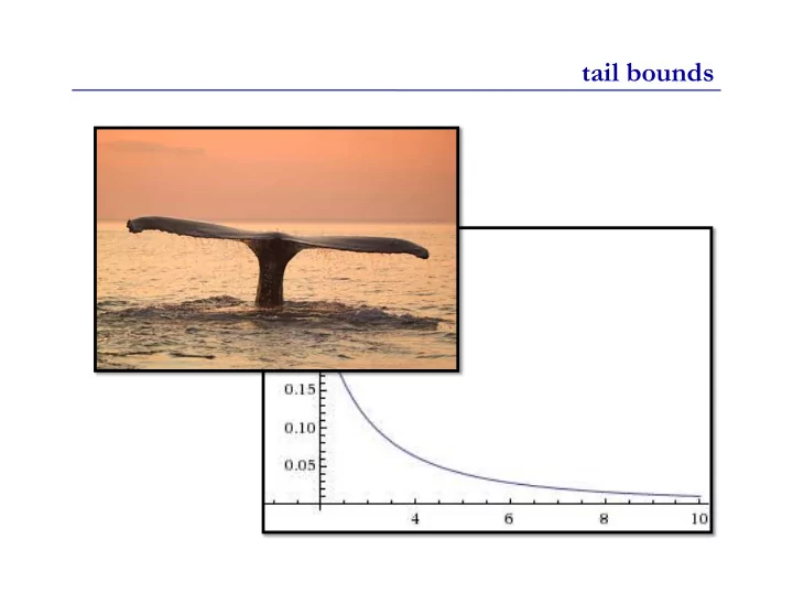
tail bounds For a random variable X, the tails of X are the parts of the PMF/density that are “far” from its mean. PMF for X ~ Bin(100,0.5) 0.08 0.06 µ ± σ P(X=k) 0.04 0.02 0.00 30 40 50 60 70 4 k

tail bounds Often, we want to bound the probability that a random variable X is “extreme.” Perhaps: 10

applications of tail bounds If we know the expected advertising cost is $1500/day, what’s the probability we go over budget? By a factor of 4? I only expect 10,000 homeowners to default on their mortgages. What’s the probability that 1,000,000 homeowners default? We know that randomized quicksort runs in � O(n log n) expected time. But what’s the probability that it takes more than 10 n log(n) steps? More than n 1.5 steps? 11

the lake wobegon fallacy “Lake Wobegon, Minnesota, where all the women are strong, � all the men are good looking, � and � all the children are above average…” 12

Markov’s inequality In general, an arbitrary random variable could have very bad behavior. But knowledge is power; if we know something , can we bound the badness? Suppose we know that X is always non-negative. Theorem: If X is a non-negative random variable, then for every α > 0, we have Corr: P ( X ≥ α E [ X ]) ≤ 1 / α 13

Markov’s inequality Theorem: If X is a non-negative random variable, then for every α > 0, we have Example: if X = daily advertising expenses and E[X] = 1500 Then, by Markov’s inequality, 14

Markov’s inequality Theorem: If X is a non-negative random variable, then for every α > 0, we have Proof: E[X] = Σ x xP(x) = Σ x< α xP(x) + Σ x ≥α xP(x) ≥ 0 + Σ x ≥α α P(x) (x ≥ 0; α ≤ x) = α P(X ≥ α ) 16

Markov’s inequality Theorem: If X is a non-negative random variable, then for every α > 0, we have Proof: E[X] = Σ x xP(x) = Σ x< α xP(x) + Σ x ≥α xP(x) ≥ 0 + Σ x ≥α α P(x) (x ≥ 0; α ≤ x) = α P(X ≥ α ) 17

Chebyshev’s inequality If we know more about a random variable, we can often use that to get better tail bounds. Suppose we also know the variance. Theorem: If Y is an arbitrary random variable with E[Y] = µ , then, for any α > 0, 18

Chebyshev’s inequality Theorem: If Y is an arbitrary random variable with µ = E[Y], then, for any α > 0, Proof: X is non-negative, so we can apply Markov’s inequality: 19

Chebyshev’s inequality Theorem: If Y is an arbitrary random variable with µ = E[Y], then, for any α > 0, Proof: X is non-negative, so we can apply Markov’s inequality: 20

Chebyshev’s inequality E.g., suppose: Y = money spent on advertising in a day E[Y] = 1500 Var[Y] = 500 2 (i.e. SD[Y] = 500) 21

Chebyshev’s inequality Theorem: If Y is an arbitrary random variable with µ = E[Y], then, for any α > 0, Corr: If Then: 23

super strong tail bounds Y ~ Bin(15000, 0.1) µ = E[Y] = 1500, σ = √ Var(Y) = 36.7 1. P(Y ≥ 6000) = P(Y ≥ 4 µ ) ≤ ¼ (Markov) 2. P(Y ≥ 6000) = P(Y- µ ≥ 122 σ ) ≤ 7x10 -5 (Chebyshev) 3. P(Y ≥ 6000) < 10 -1600 (Y ~ Poi(1500)) < < < 4. The exact (binomial) value is ≈ 4 x 10 -2031 1,2,5 are easy calcs; 3 & 4 are not (underflow, etc.) 5. P(Y ≥ 6000) ≲ 10 -1945 (Chernoff, below; easy) 26

Chernoff bounds Method: B&T pp 284-7 Suppose X ~ Bin(n,p) µ = E[X] = pn Chernoff bound: 27

Chernoff bounds B&T pp 284-7 Suppose X ~ Bin(n,p) µ = E[X] = pn Chernoff bound: 28

router buffers 29

router buffers Model: n = 100,000 computers each independently send a packet with probability p = 0.01 each second. The router processes its buffer every second. How many packet buffers so that router drops a packet: • Never? 100,000 • With probability ≈ 1/2, every second? ≈ 1000 (P(X>E[X]) ≈ ½ when X ~ Binomial(100000, .01)) • With probability at most 10 -6 , every hour? 1257 • With probability at most 10 -6 , every year? 1305 • With probability at most 10 -6 , since Big Bang? 1404 Exercise: How would you formulate the exact answer to this problem in terms of binomial probabilities? Can you get a numerical answer? 30

router buffers X ~ Bin(100,000, 0.01), µ = E[X] = 1000 Let p = probability of buffer overflow in 1 second By the Chernoff bound p = Overflow probability in n seconds � = 1-(1-p) n ≤ np ≤ n exp(- δ 2 µ/3) , which is ≤ ε provided δ ≥ √ (3/ µ )ln( n / ε ). For ε = 10 -6 per hour: δ ≈ .257, buffers = 1257 For ε = 10 -6 per year: δ ≈ .305, buffers = 1305 For ε = 10 -6 per 15BY: δ ≈ .404, buffers = 1404 32

summary Tail bounds – bound probabilities of extreme events Important, e.g., for “risk management” applications Three (of many): Markov: P(X ≥ k µ ) ≤ 1/k (weak, but general; only need X ≥ 0 and µ ) Chebyshev: P(|X- µ | ≥ k σ ) ≤ 1/k 2 (often stronger, but also need σ ) Chernoff: various forms, depending on underlying distribution; usually 1/exponential, vs 1/polynomial above Generally, more assumptions/knowledge ⇒ better bounds “Better” than exact distribution? Maybe, e.g. if latter is unknown or mathematically messy “Better” than, e.g., “Poisson approx to Binomial”? Maybe, e.g. if you need rigorously “ ≤ ” rather than just “ ≈ ” 34