T HE Internet of Things (IoT) is characterized by the utilization - - PDF document

SLIDE 1

1

Modeling Compound TCP over WiFi for IoT

Shiva Raj Pokhrel and Carey Williamson

Abstract—Compound TCP will play a central role in future home WiFi networks supporting Internet of Things (IoT) ap-

• plications. Compound TCP was designed to be fair, but can

manifest throughput unfairness in infrastructure-based IEEE 802.11 networks when devices at different locations experience different wireless channel quality. In this paper, we develop a comprehensive analytical model for Compound TCP over WiFi. Our model captures the flow and congestion control dynamics

• f multiple competing long-lived Compound TCP connections,

as well as the Medium Access Control (MAC) layer dynamics (i.e., contention, collisions, and re-transmissions) that arise from different Signal-to-Noise Ratio (SNR) perceived by the devices. Our model provides accurate estimates for TCP packet loss probabilities and steady-state throughputs for IoT devices with different SNR. More importantly, we propose a simple adaptive control algorithm to achieve better fairness without compromising the aggregate throughput of the system. The proposed real- time algorithm monitors the access point queue and drives the system dynamics to the desired operating point, which mitigates the adverse impacts of SNR differences, and accommodates the sporadically-transmitting IoT sensors in the system. Keywords—Internet of Things, Compound TCP, fixed-point anal- ysis, WiFi, throughput unfairness, adaptive control.

I. INTRODUCTION

T

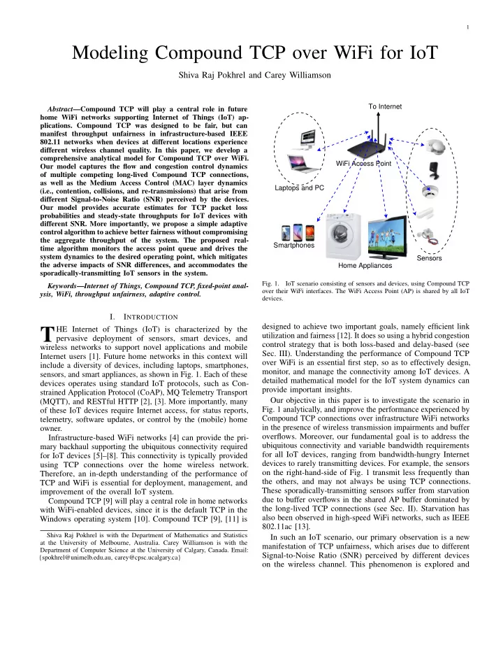
HE Internet of Things (IoT) is characterized by the pervasive deployment of sensors, smart devices, and wireless networks to support novel applications and mobile Internet users [1]. Future home networks in this context will include a diversity of devices, including laptops, smartphones, sensors, and smart appliances, as shown in Fig. 1. Each of these devices operates using standard IoT protocols, such as Con- strained Application Protocol (CoAP), MQ Telemetry Transport (MQTT), and RESTful HTTP [2], [3]. More importantly, many

• f these IoT devices require Internet access, for status reports,

telemetry, software updates, or control by the (mobile) home

• wner.

Infrastructure-based WiFi networks [4] can provide the pri- mary backhaul supporting the ubiquitous connectivity required for IoT devices [5]–[8]. This connectivity is typically provided using TCP connections over the home wireless network. Therefore, an in-depth understanding of the performance of TCP and WiFi is essential for deployment, management, and improvement of the overall IoT system. Compound TCP [9] will play a central role in home networks with WiFi-enabled devices, since it is the default TCP in the Windows operating system [10]. Compound TCP [9], [11] is

Shiva Raj Pokhrel is with the Department of Mathematics and Statistics at the University of Melbourne, Australia. Carey Williamson is with the Department of Computer Science at the University of Calgary, Canada. Email: {spokhrel@unimelb.edu.au, carey@cpsc.ucalgary.ca} WiFi Access Point Smartphones Laptops and PC To Internet Sensors Home Appliances

• Fig. 1.

IoT scenario consisting of sensors and devices, using Compound TCP

• ver their WiFi interfaces. The WiFi Access Point (AP) is shared by all IoT

devices.

designed to achieve two important goals, namely efficient link utilization and fairness [12]. It does so using a hybrid congestion control strategy that is both loss-based and delay-based (see

• Sec. III). Understanding the performance of Compound TCP
• ver WiFi is an essential first step, so as to effectively design,

monitor, and manage the connectivity among IoT devices. A detailed mathematical model for the IoT system dynamics can provide important insights. Our objective in this paper is to investigate the scenario in

• Fig. 1 analytically, and improve the performance experienced by

Compound TCP connections over infrastructure WiFi networks in the presence of wireless transmission impairments and buffer

• verflows. Moreover, our fundamental goal is to address the

ubiquitous connectivity and variable bandwidth requirements for all IoT devices, ranging from bandwidth-hungry Internet devices to rarely transmitting devices. For example, the sensors

• n the right-hand-side of Fig. 1 transmit less frequently than

the others, and may not always be using TCP connections. These sporadically-transmitting sensors suffer from starvation due to buffer overflows in the shared AP buffer dominated by the long-lived TCP connections (see Sec. II). Starvation has also been observed in high-speed WiFi networks, such as IEEE 802.11ac [13]. In such an IoT scenario, our primary observation is a new manifestation of TCP unfairness, which arises due to different Signal-to-Noise Ratio (SNR) perceived by different devices

• n the wireless channel. This phenomenon is explored and

SLIDE 2

2

500 1000 1500 2000 Time in Seconds 20 40 60 80 100 Buffer Occupancy (number of packets)

• Fig. 2.

AP buffer occupancy (in packets) with four Compound TCP

• connections. The AP buffer is almost always full.

explained in greater detail in the next section. The primary contributions in this paper are two-fold:

• We develop a comprehensive analytical model that can

accurately capture the throughput of Compound TCP connections over an 802.11 infrastructure WLAN with wireless channel errors (Sec. IV). Our model explains the

• bserved download-download unfairness due to different

SNR perceived by the IoT devices. The accuracy of our model is validated by extensive simulations.

• Based on the insights provided by our analytical model,

we develop an adaptive algorithm that appropriately manages the AP buffer and eliminates starvation and ameliorates throughput unfairness over WiFi. Our Virtual Buffer Sharing (VBS) algorithm guarantees ubiquitous connectivity among the devices and provides a mecha- nism to satisfy the variable bandwidth requirements of IoT devices. We perform extensive evaluation of the VBS algorithm for the IoT scenario in Fig. 1. The appendix provides a control-theoretic analysis of the system dynamics highlighting the existence, stability, and convergence of Compound TCP dynamics over WiFi with the VBS algorithm. At a higher conceptual level, our work provides a technical feasibility analysis of WiFi-enabled sensors for IoT. A key finding is that for stability of overall system dynamics, the Compound TCP parameters will possibly have to be jointly designed with the VBS algorithm parameters (see Appendix). The remainder of the paper is organized as follows. Sec. II provides a motivating example for our work, using ns-2 network simulation. In Sec. III, we explain the mechanisms

• f Compound TCP, and discuss our network scenario in detail.

Our model for describing the download-download throughput unfairness due to wireless errors is developed in Sec. IV. Our solution to achieve throughput fairness by buffer management is provided in Sec. V. Results from our analytical model and buffer management algorithm are validated with ns-2 simulation [14] results in Sec. VI. Sec. VII summarizes prior related work, and

• Sec. VIII discusses future directions in wireless technology.
• Sec. IX concludes the paper, with the control-theoretic analysis
• f system dynamics deferred to the appendix.

II. MOTIVATING EXAMPLE This section presents a simple simulation experiment illus- trating the TCP unfairness and starvation problem in our IoT scenario (see Fig. 1). This scenario serves as a motivating example for our work, and also provides key insights into our proposed model and solution. Our simulated scenario considers four IoT devices down- loading data over the home wireless network, using long- lived Compound TCP connections. We assume that two of the devices have excellent wireless channel quality, while two have poorer connectivity. Our discussion focuses on the throughputs achieved by these connections, and their fairness, in the presence of packet losses from either: (i) buffer overflows at the DropTail AP buffer; or (ii) MAC-layer losses and collisions.

• A. AP Buffer Overflow

The first main observation in this scenario is that when there are multiple TCP connections, the AP buffer is almost always full (see Fig. 2). With at least two IoT devices, and realistic round-trip propagation delays, the AP buffer of WiFi is the bottleneck because TCP always tends to fill the link capacity and any available buffers [15], [16]. This observation is not all that surprising, given that the WiFi link is typically the bottleneck compared to the external Internet bandwidth in a download-intensive home network [17]. Furthermore, most TCP versions grow the congestion window until receiving a packet loss signal. Thus losses from AP buffer overflow occur in this scenario. Under non-zero wireless channel errors, the TCP data packets

• f all the users must be served by the AP, but the WiFi

standard does not provide prioritized access for the AP. So, most outstanding TCP data packets queue up at the AP buffer and only a few are at user devices (about 1.5 packets on average [18], [19]). Moreover, in our network scenario where

• nly a subset of the devices suffer from channel errors, the AP

buffer is nearly always full. This creates a starvation effect for the sporadically-transmitting IoT sensors, which may find the AP buffer full, leading to buffer overflows. The impacts of buffer overflows are different for upload and download connections [16], [20]–[25]. In particular, download connections lose TCP DATA packets and upload connections lose TCP acknowledgements (ACKs). Since TCP ACKs are cumulative, their loss does not have significant adverse impact

• n the upload connections. The loss of TCP DATA packets,

however, must be recovered by TCP-level retransmission, and sometimes may lead to time-outs. This results in a (multi- plicative) decrease of the congestion window of the download

• connections. Hence, upload connections typically obtain a

higher share of the throughput than download connections [16], [20]–[26].

SLIDE 3

3

50 100 150 200 250 300 350 400

Time in seconds

2 4 6 8 10 12

Individual Throughput, , Mbps

• pw=0.0
• pw=0.3
• pw=0.0
• pw=0.3
• Fig. 3.

Throughput unfairness between four Compound TCP connections

• ver WiFi as observed in ns-2 simulations due to difference in wireless error

probability pw.

• B. MAC-layer Effects

The second form of losses are those due to collisions and wireless channel errors [19], [27], [28]. In our home WiFi scenario, the overall signal-to-noise ratio (SNR) perceived by upload connections can be significantly worse than that for download connections, since the AP is almost always contending for the channel with uploading devices [19], [28]. Packet losses can result in a (multiplicative) decrease of the congestion window of the upload connections. Hence, download connections obtain a higher share of the throughput than upload connections. The degree of unfairness increases as the probability of wireless errors increases. The key observation in this simulation scenario is that Com- pound TCP leads to throughput unfairness in an infrastructure WiFi network due to the SNR differences perceived by the downloading devices (see Fig. 3). Specifically, under non- zero wireless channel errors, downloading connections with higher SNR can achieve higher throughput than downloading connections with lower SNR. Moreover, the degree of this unfairness increases as the SNR difference increases. This type

• f unfairness has been observed in experiments [29] and studied

in [27]. As the difference in SNR between any two devices increases, an IoT device with lower SNR obtains a much smaller through- put as compared to the other devices with higher SNR. Unlike in the upload-download case where unfairness occurs due to the loss of TCP DATA packets by the downloading devices, the unfairness in this case of Compound TCP downloads is due to the following: 1) Compound TCP is able to distinguish between packet losses due to congestion and packet losses due to channel errors but unable to distinguish the difference in losses perceived by the co-existing TCP flows. 2) Devices with lower SNR have a smaller TCP congestion window, and thus fewer packets in the AP buffer. The evolution of TCP congestion windows observed in simulations is illustrated in Fig. 4. 3) FIFO queuing at the AP buffer results in each device get- ting a throughput share proportional to their occupancy

• f the shared AP buffer.

It is worth noting that the well-known SNR-aware rate adap- tation approach, which dynamically changes the transmission rate to adapt to the time-varying channel quality, is not useful

• here. This is because for competing TCP flows sharing the

same AP, the auto-rate fallback mechanism will further decrease the data rate of the device with lower SNR providing more AP buffer space for the packets belonging to the higher SNR devices, which is not desirable. Therefore, for tractability of the proposed model and solution, auto-rate adaptation is disabled in the analysis and experiment of this paper (similar to that in [19], [27]).

• C. Modeling Insights

As will be discussed in Section VII, existing analytical models do not capture the throughput unfairness of Compound TCP due to the difference in wireless channel errors. Our model is designed to capture SNR differences among devices, and its interplay with the loss-based and delay-based congestion control mechanisms of Compound TCP. This requires a different and rigorous mathematical approach. We adopt a flexible and scalable approach while developing the analytical models, and then follow the fixed-point approach [30] for independent component analysis. Another key insight is that the buffering at the AP must be monitored and appropriately managed to eliminate starvation and ameliorate unfairness caused by SNR differences and wireless channel errors. Specifically, we need to control queue

• ccupancy and keep some space available for rarely arriving

packets at the AP buffer. This can be guaranteed by monitoring the queue and maintaining it below the maximum available AP buffer capacity.

50 100 150

Time in seconds

5 10 15 20 25 30 35

Congestion windows in packets

Window-pw=0.3 Window-pw=0.0

• Fig. 4.

Evolution of the TCP congestion windows with Wmax = 45, Bap = 100 packets and wireless error probability pw.

SLIDE 4

4

In the absence of wireless channel errors, the throughput unfairness between uploads and downloads due to buffer

• verflows can be balanced by simply increasing the buffer

capacity at the AP. In general, the larger the AP buffer is, the fairer is the throughput share. We, however, argue that since wireless channel errors are indeed unavoidable in real networks, increasing the AP buffer beyond a certain value simply leads to another type of unfairness. Instead, the AP buffer should be managed appropriately such that the adverse impact of buffer losses would counter-balance the adverse impact of wireless channel errors, so that the resulting throughputs are fair. In fact, we need a global solution for all types of unfairness observed so far, to provide the performance required for the deployment

• f IoT using WiFi.

These key insights lead to our second main contribution, namely an adaptive algorithm that appropriately manages the AP buffer and eliminates the starvation and throughput unfairness in WiFi. The proposed AP buffer management algorithm can be implemented by logical buffer partitioning, referred to as Virtual Buffer Sharing (VBS) in this paper, which uses the memory management concept from operating systems [31] (Sec. V). In particular, our real-time algorithm always maintains the buffer occupancy at the AP slightly below the full capacity, and partitions the AP buffer properly to ensure fairness (Sec. VI-C). Furthermore, VBS does so without compromising the aggregate throughput of the system. Our solution can be deployed at the AP and is compatible with the existing TCP/IP protocols and WiFi standards [4]. The end result is that our VBS algorithm makes the IoT system realizable with WiFi networks. The remaining sections provide further details on our model and its evaluation. III. COMPOUND TCP, NETWORK SETTING AND ASSUMPTIONS

• A. Compound TCP

Compound TCP is a hybrid transport-layer protocol that uses both packet loss and round trip time (RTT) as feedback signals in order to operate its flow and congestion control

• mechanisms. The loss-based congestion window, Wloss, is the

same as in the standard TCP Reno algorithm while the delay- based window, Wdelay, considers the additional feedback about the network delay characteristics. The effective congestion window of Compound TCP is computed as [9] W = min{Wloss + Wdelay, Wmax} where Wmax is the maximun advertised receiver window for managing the flow control. This prevents overwhelming the receiver buffer of IoT devices in our scenario. By keeping track of the minimal RTT observed so far, called the base round trip time (RTTb), Compound TCP maintains a variable dif which is updated as, dif = RTTb( W RTTb − W RTT ). In fact, this is the difference between expected sending rate (for the base round trip time) and actual sending rate, which

To Internet Wireless link Wireline link AP STA

• Fig. 5.

An infrastructure WLAN consisting of an AP and N downloading

• STAs. The STAs communicate with servers in the Internet through the AP

using long-lived Compound TCP connections. The servers are connected to the AP by high-speed wired links with negligible delay.

gives an estimate of the number of packets backlogged in the network buffer. The Compound TCP congestion window update algorithm is [10], W i+1 =    (W i + 1 + (α(W i)κ − 1)+), if dif < th (W i + 1 − ζdif), if dif > th

W i

loss

2

+ W i

delay(1 − β), if loss

(1) In this formulation, the parameters α, β, κ are the scalability, smoothness, and responsiveness parameters of the Compound TCP window update function, and their typical values are α = 0.125, β = 0.5, κ = 0.75 [9]. Furthermore, (.)+ means max(., 0), ζ > 0, and th is the minimum threshold indicating the number

• f backlogged packets required to detect congestion to quantify

the tradeoff between throughput and buffer requirement for TCP fairness. We use th = 30 packets as in [9]. Congestion is detected when the number of packets in the queue is larger than a threshold th. Observe in Equation (1), if dif < th, the path is underutilized; otherwise, the path is considered as busy and the delay-based component would gracefully reduce its window. Consider the case of a packet loss that occurs when dif < th; it is highly probable that the loss is due to channel errors rather than due to buffer

• verflows, since the path is underutilized. This observation

means that Compound TCP could distinguish between buffer and channel losses. However, both types of losses are interpreted as congestion by Compound TCP (see last step of Equation (1)).

• B. Network Settings and Mechanisms

We develop an IoT scenario using 802.11 infrastructure WLAN as depicted in Fig. 5 (similar to Fig. 1). There are N devices downloading through the AP using long-lived Compound TCP connections. The AP and devices use the standard Distributed Coordination Function (DCF) of the Medium Access Control (MAC) protocol [4]. The external servers outside the WLAN are connected to the AP using

SLIDE 5

5

high-speed links with minimal delay. The wireless channel from the AP to the STAs is the bottleneck. This is due to the closed-loop nature of TCP: most TCP DATA packets are at the AP buffer waiting for service, on average only few devices are contending (i.e., have Compound TCP ACKs in their queues and sense for channel access) irrespective of how many devices are associated with the AP [19], [20], [32]. 1 Each TCP packet (i.e, a Compound TCP DATA or ACK) is encapsulated into one MAC frame and is transmitted between the AP and the stations using the DCF MAC protocol. Frame transmissions occasionally fail due to collisions and/or wireless

• errors. When there are two or more nodes (i.e., AP or device)

attempting transmission in the same slot, a collision occurs [33]. In the DCF MAC protocol, every unsuccessful transmission is interpreted as a collision even though it might fail due to wireless errors. After each transmission failure (detected by the absence of a MAC-level ACK), the MAC contention window is doubled (maximum allowed value m). The packet is retransmitted up to k times. A TCP packet is discarded if all k re-transmissions for the same packet fail. To overcome the influence of BER, MAC frames are protected with Forward Error Correction (FEC) that can recover data up to a certain level of BER. The MAC frames carrying Compound TCP ACKs are small, and due to FEC, they are rarely lost under realistic channel errors. Moreover, since Compound TCP ACKs are cumulative, the loss of a few Compound TCP ACKs does not have an adverse impact. Compound TCP DATA packets, however, are large enough to suffer from channel errors. We consider the impact of correlated buffer loss and wireless channel errors. A Compound TCP DATA packet that is lost due to buffer overflow at the AP will not be further dropped at the MAC due to re-transmission failures. However, lost packets (irrespective of the causes) have to be recovered by TCP-level re-

• transmission. This loss of a Compound TCP DATA packet either

due to buffer overflow or due to MAC discard is interpreted by the Compound TCP source as an indication of congestion. The detection of the loss of a Compound TCP DATA packet

• ften leads to a multiplicative decrease of Compound TCP’s

congestion window. We make two simplifying assumptions in our analysis: 1. The AP is always backlogged with packets and contend- ing for the channel (saturated AP). Saturation of AP with TCP flows is observed in simulation as depicted in Fig. 2 and also in practice [16], [21]. TCP flows are mostly in the congestion avoidance phase with approximately every received ACK triggering one new TCP packet from the TCP source. Due to this principle within TCP, a device’s MAC queue sends a TCP ACK only after it receives a TCP DATA packet from the AP. Indeed, a single AP has to serve all IoT devices, but under DCF, the AP and IoT devices all have equal

• pportunity of channel access. Thus, one AP competing with

several IoT devices in the WiFi means that most of the packets are backlogged at the AP buffer for service.

1We consider the downloading scenario in this paper for simplicity. However,

the analysis can be extended for the case of both uploads and downloads along the lines of [19], [20].

2. The impact of transmission failure or discard of Com- pound TCP ACKs and MAC-level ACKs due to wireless channel errors is negligible. TCP ACKs are cumulative; when a TCP sink acknowledges that it correctly received a DATA packet in a TCP flow, it implicitly informs the source that all of the previous DATA packets were received correctly. It uses cumulative acknowledgment scheme with its TCP sliding window. In contrast, most MAC protocols use a stop-and-wait mechanism; they transmit the next packet from the queue only if the current packet has been properly acknowledged (no sliding window mechanism like in TCP). MAC protocols use positive ACKs and MAC level retransmissions to avoid losing packets on the medium. The principle of MAC is quite simple: each time a device/AP receives a packet, it sends back immediately an ACK to the sender to indicate that it has successfully received the packet without errors. If the sender doesn’t receive an ACK, it presumes that the packet was lost, so it will retransmit the packet (after contending again for the medium). The reasoning is that it makes the protocol simpler, minimizes latency, and avoids reordering packets. Also the MAC frames containing both types

• f ACKs are so small that, with FEC, they are seldom lost

under realistic wireless errors. IV. MODELING COMPOUND TCP WITH WIFI AND IOT

DEVICES

Figure 6 provides a structural overview of our Compound TCP model, which has seven components. While some of these components borrow heavily from prior published models, others are new. Furthermore, to the best of our knowledge, ours is the first approach to assemble all of these components together into a comprehensive model for Compound TCP over WiFi. 1) Non-Markovian Analysis: In contrast to prior related work [19], [27], we use a simple non-Markovian analysis to compute the throughput and loss perceived by IoT devices in the WiFi system, by combining it with the Compound TCP dynamics of (1). The Markovian approach for non-saturated WiFi analysis along the lines of [19], [27], [34] could be intractable for realistically sized network and IoT devices of Fig. 1, because

• f the prohibitively large dimensionality and complexity arising

due to the different SNR classes. Therefore, we adopt a simple yet novel approach, which significantly reduces the complexity

• f the TCP-controlled WiFi analysis. This is based on the

rate equilibrium principle for TCP data transfer: when TCP’s delayed ACK mechanism is disabled, the average rate of downlink TCP DATA packets (packets/sec) from the AP is proportional to that of uplink TCP ACKs (packets/sec) from the IoT devices. 2 2) Fixed-point method: We decompose the analysis of different aspects of the system behavior into different modules. The different components of our overall analytical model work independently and their inter-dependencies are shown in Fig. 6. The closed-form expressions for each component are derived by assuming that the quantities used as inputs from the other

2When the delayed ACK mechanism is enabled, the number of TCP ACKs

is reduced by the delayed ACK factor, which is typically 2.

SLIDE 6

6

blocks (outputs) are already computed. All blocks are finally coupled using fixed-point equations. Table I summarizes the notation used for our model. Next, we explain each of the seven components of Fig. 6 in detail.

TABLE I. MODEL NOTATION.

Given Inputs ni Total number of IoT devices in SNR class i k Maximum MAC-layer retransmissions per packet, k = 7 m Maximum number of MAC failures for which the WiFi contention window is doubled, m = 5 pw Probability that a MAC frame will suffer from wireless channel error for SNR class i. h∗

i

Desired fraction of service by the AP for Compound TCP data packets in SNR class i. For example, if the desired throughput ratio is 1.11, then h∗

i

= 0.526 (for two classes). Wmax Maximum receive window for Compound TCP Bap Size of the AP buffer in packets Internal Variables hi Fraction of services by the AP that are Compound TCP data packets belonging to SNR class i, i.e. Probability that Head

• f Line (HOL) packet at the AP belongs to an IoT device
• f SNR class i

βap Average probability of a TCP DATA packet from the AP βi Average probability of TCP ACK packet from IoT devices E[X] Expected duration between two consecutive services of packets (frames) in MAC fap Aggregate failure probability during service of Compound TCP data packet from the AP fi Aggregate failure probability during service from IoT de- vices pd,i Probability of TCP packet discard/drop at the MAC layer from IoT device of SNR class i pm Probability of packet loss as perceived by TCP source due to combined impact of buffer overflow, wireless loss, and collisions Outputs pb Probability with which packets arriving at the AP buffer encounter loss due to buffer overflow pi Blocking probability with which packets arriving at the AP buffer are dropped by the VBS algorithm Θi Aggregate throughput (in packets/second) of Compound TCP flows for IoT devices belonging to SNR class i

• A. Compound TCP Window Analysis

Let the congestion window of any Compound TCP con- nection be denoted by ˜

• Ww. The integer part of ˜

Ww, hence- forth called the congestion window, is denoted by Ww, i.e., Ww = ⌊ ˜ Ww⌋. Then, given that there is no loss, the increment in congestion window per received ack, δ(Ww), can be computed using (1) as [10], δ(Ww) = α(Ww)κ. (2) Note that the AP buffer is shared between several connections from the IoT devices. A connection from a device can experience packet losses due to the AP buffer being largely filled with the packets belonging to other devices. Let pm denote the overall packet loss probability perceived by the TCP source due to buffer overflows at the AP, wireless channel errors, and MAC-layer collisions. The congestion window Ww increases by one from ℓ to ℓ+1, if and only if (δ(ℓ))−1 packets are successfully transferred to the destination3, i.e., they are not

3The δ(ℓ) for the case of Compound TCP can be viewed as 1 w in the case

• f TCP Reno with a congestion window of w packets. The idea used in (3) is

similar: w packets need to be successfully acknowledged before the congestion window of TCP Reno can increase from w to w + 1 [35].

MAC Saturation Analysis (Sec. IV-B2) pb Computation Compound TCP Window Analysis (Sec. IV-A) Buffer Loss Analysis (Sec. IV-C2) Compound TCP Throughput Analysis (Sec. IV-B1) Failure and Drop Analysis (Sec. IV-B4) Rate Equilibrium Analysis (Sec. IV-B3) Head of Line Analysis (Sec. IV-C1)

pd,i βap pd,i hi pd,i pw E[Wi] Bap E[Xi], fi fap,i pb βi βap,i Θi

• Fig. 6.

Components and relationships in our Compound TCP model.

lost due to any cause; otherwise, Ww reduces to half its value, i.e., from ℓ to ⌈ ℓ

2⌉. Let the changes in Ww occur at times {Yn},

n = 1, 2, 3, . . . , and let Ww(n) denote the congestion window immediately after the change has occurred at time Yn. Let Wmax denote the receiver advertised window. Then, the Compound TCP congestion window evolution process {Ww(n), n ≥ 0} can be modelled as a Discrete Time Markov Chain (DTMC) with the state space {1, 2, 3, ...., Wmax} and its state transition probabilities are given by Pr (Ww(n + 1) = ℓ + 1 | Ww(n) = ℓ) = (1 − pm)(δ(ℓ))−1, Pr (Ww(n + 1) = ⌈ℓ/2⌉ | Ww(n) = ℓ) = 1 − (1 − pm)(δ(ℓ))−1. (3) Given the overall packet loss probability pm (combined impact of buffer overflows and MAC discards), the stationary distribution of the DTMC {Ww(n), n ≥ 0}, denoted by Πw(·), can be numerically computed. Then, the expected congestion window, E[Ww], can be obtained as E[Ww] =

Wmax

• ℓ=1

ℓΠw(ℓ). (4)

• B. MAC Layer Analysis

In this section, we develop the modules for TCP controlled WiFi throughput and MAC level loss. 1) Computation of Compound TCP Throughput: The DCF backoff mechanism in WiFi [4] imposes a so-called slotted

• structure. Consider σ the duration of an idle slot, Tdata is

the duration occupied by the TCP DATA transmission, and

SLIDE 7

7

Tack is the duration occupied by the Compound TCP ACK transmission (all in seconds). Let St,i denote the total number

• f Compound TCP ACK packets successfully transmitted by

the device in SNR class i after t seconds. Then the aggregate device throughput, Θi, for SNR class i is given by Θi = lim

t→∞

St,i t ≈ βi(1 − fi) E[X] , (5) where i) βi, fi is the expected attempt and failure probabilities of all the IoT devices with the same SNR (suffering from channel error pw). ii) E[X] is the expected duration between two consecutive services of packets in the MAC. The E[X] can be computed as E[X] := P0σ + PsTack + PlTdata (6) where i) X is a random variable that represents time between two services (successful or failure); ii) P0 is the probability that a slot is idle; iii) Ps is the probability that a slot is successful transmission

• f TCP ACK (or failure of TCP ACK due to collision

and/or channel errors); and iv) Pl is the probability that a slot is successful transmission

• f TCP DATA (or failure involving at least one TCP

DATA packet due to collision and/or channel errors). The aforementioned probabilities are computed as fol- lows [33], P0 = (1 − βap)

• i

(1 − βi)ni, (7) Ps = (1 − βap)(1 −

• i

(1 − βi)ni(1 − pw)), and (8) Pl = 1 − P0 − Ps. (9) where i) βap is the expected attempt probability of an AP; and ii) ni is the total number of devices with the same SNR. Remark IV.1. Our analysis can be extended to handle rate heterogeneity among the IoT devices. Then the computation of E[X] in (6) must be modified by substituting the appropriate values of the times T i

data and T i ack for successful transmission of

TCP DATA and TCP ACK packets, respectively, corresponding to the physical rate ri of a device belonging to SNR class i. 2) Computation of Attempts and Collision Probabilities: Recall that the AP is saturated and is always contending for the MAC channel (Assumption 1). The transmission attempt probability of a packet from the AP can be computed by using fixed-point function, G(.), using saturation contention analysis (quite similar to [33]), βap = G(fap) (10) where fap is the expected (conditional) failure probability of a transmission from the AP due to collisions and/or channel errors for all of the IoT devices. 3) Rate Equilibrium Analysis: The transmission attempt probability of a TCP DATA packet from the AP belonging to any IoT device in a network is proportional to the fraction of its packets inside the AP buffer. Therefore, given the fraction hi of packets in the AP buffer from SNR class i, the attempt probability of a packet belonging to those devices from the AP is βap,i = hiβap (11) On the reverse path, the combined effort of all of the IoT devices is to transmit TCP ACKs corresponding to the successfully received TCP DATA packets from the AP. Therefore, the attempt probability βi of a TCP ACK from the IoT devices in SNR class i, and that from the AP to those devices, βap,i satisfy the following equilibrium condition, E[Attempts of TCP DATA packets, SNR class i]βap,i = E[Attempts of TCP ACK packets of SNR class i]βini So, βi = E[Attempts of TCP DATA packets, SNR class i]βap,i E[Attempts of TCP ACK packets of SNR class i]ni = (1 − fap)(1 − (fi)k+1)βap,i (1 − fi)(1 − (fap)k+1)ni (12) Note that our analysis even handles the case when all of the IoT devices have different SNR, i.e. when ni = 1 and all IoT devices observe different loss rates. The conditional failure probabilities fap and fi are given by fap = 1 −

• i

(1 − βi)ni(1 − pw) (13) fi = 1 − (1 − βap)(1 − βi)(ni−1)

• j=i

(1 − βj)nj (14) 4) Packet Discard/Drop Analysis: The failure probability for the TCP DATA packets transmitted from the AP can be computed by using fixed-point function, G−1(.), with saturation contention analysis similar to (15), fap,i = G−1(βap,i) (15) As discussed earlier in (11), βap,i is the expected attempt probability from the AP to the IoT devices represented by the hi fraction of TCP DATA packets inside the AP buffer. The corresponding drop probability perceived by the Compound TCP connections from the devices is given by pd,i = (fap,i)k+1, (16) where k denotes the maximum number of MAC-layer retrans- missions allowed before discard.

• C. Cross-Layer Analysis

In this section, we track the fraction of packets inside the AP buffer using a simple cross-layer approach, and then compute the corresponding buffer loss due to overflows at the AP.

SLIDE 8

8

1) Head Of Line (HOL) Analysis: Let λi

ap denote the arrival

rate of Compound TCP DATA packets into the AP buffer for the devices with the same SNR. Then, in steady state, the probability hi that the HOL packet at the AP belongs to those IoT devices is equal to the ratio of the arrival rate of Compound TCP DATA packets belonging to those IoT devices to the total arrival rate into the AP buffer, i.e., hi = λi

ap

• j λj

ap

≈ niE[Wi]

• j njE[Wj] ≈

niΘi(1 + pd,i)

• j njΘj(1 + pd,j)

(17) The approximation in (17) is that RTT experienced by all Compound TCP connections is dominated by the queuing delay at the AP, and all IoT devices associated with the same AP experience the same RTT [15]. 2) Buffer loss Analysis: Consider a situation where the AP buffer can store up to Bap packets. Our next objective is to

• btain the probability of buffer overflow, pb. The maximum

amount of data in the network at any given point in time is given by the Bandwidth Delay Product (BDP). Based on the BDP for a single Compound TCP connection, the number of packets in the WiFi network is given by (see [36, Eqn. (2)]) BDP WiFi

in packets

≈

• i

niE[Wi] (18) We assume that the propagation delay is negligible, and that the number of packets in flight at any point in time is negligible. The number of packets at the IoT devices is also negligible because there are few IoT devices contending (1.5 on average [18], [32]). Thus, almost all of the BDP W iF i

in packets packets are

at the AP buffer. Since Compound TCP tends to fill up the available buffer, we approximate BDP W LAN

in packets with Bap and

• btain

Bap ≈

• i

nif(pb + (1 − pb)pd,i) (19) Equation (19) can be solved to obtain the average buffer loss probability at the AP, pb, for a given value of Bap. Remark IV.2 (With propagation delay). In many applications, the IoT device must operate with a very small duty cycle: wake up for several milliseconds to perform its function, transmit its data payload, and then go back to sleep. Furthermore, this applies whether the propagation delay is negligible or not. When the propagation delay is Ti seconds, the number of packets in flight for connection i is given by ΘiTi. Therefore, Equation (19) will take the form Bap +

• i

niΘiTi ≈

• i

nif(pb + (1 − pb)pd,i). (20)

• D. Fixed-Point Iteration

Define a vector x = (hi, pi) . In each iteration j of our fixed- point computation, we start at a point xj and apply Eqns. (3), (4)-(19) to obtain a new point xj+1. In our extensive numerical experiments, we observed the iterations always converge to the same solution irrespective of the initial point (see Appendix). V. ADAPTIVE VBS ALGORITHM In this section, we use the idea of buffer partitioning from

• perating systems [31, pp. 300-307]. We perform virtual

partitioning of the AP buffer and provide the desired share of buffer to each of the IoT devices depending upon their SNR and/or bandwidth requirements. We apply the insights from

• ur HOL analysis of the model, to manage the AP buffer so

that a desired ratio of throughput, and thus, a desired degree of throughput fairness, may be achieved by controlling the share at the AP buffer. To achieve a specific throughput ratio, rather than fixing the buffer share for each device a priori, we apply h∗

i as a given

constant when solving the fixed-point equations and obtain the converged values. A software patch at the AP could easily handle the VBS algorithm and is compatible with the existing WiFi standards and TCP protocols (see Algorithm 1). In fact, the desired throughput ratio can be achieved by adopting the following two approaches at the AP: 1. Unfairness Solution: Admit each arriving packet into the AP buffer with probability 1 − pi(h∗

i ), and block

with probability pi(h∗

i ).

2. Starvation Solution: Maintain the AP buffer occupancy Q(t) := cBap; where c is a positive constant, 0.5 < c < 1. We use c = 0.6 and Q(t) :=

i ni(t)E[Wi]

(see (20)) in our numerical experiments. In particular, our objective is to min (Q(t) − cBap)2. Algorithm 1 VBS Algorithm at AP

1: procedure INITIALIZE 2: Desired fraction (h∗

i ), Buffer Size (Bap)

3: end procedure 4: procedure UPDATE 5:

while ((Qn − cBap)2 > tol) do

6:

if (hi(n) < h∗

i ) then pi(n) = 0.0

7:

else pi(n) = 1.0

8:

end if

9: Obtain hi(n) and Qn 10:

end while

11: end procedure

When the wireless channel impairment or number of users changes over time, the blocking probabilities pi(t) should adapt

• accordingly. Consider that the 802.11 network is operating in

steady state and the throughput ratio is at the desired value

• f h∗

i . When the magnitude of wireless channel impairment

pw(t) changes, with the old value of blocking probability, the throughput ratio will start deviating from the target value and will have new value hi(t) (locally observable at AP). The VBS algorithm uses this deviation to steer the network to the required h∗

i by renewing the value of pi(hi(t)) automatically.

The algorithm tracks the AP buffer occupancy Q(t) (locally

• bservable at AP), and ensures that it remains below the total

capacity Bap. This approach eliminates the starvation problem, by providing enough room for sporadically-transmitting devices. The proposed Algorithm 1 is generic and dynamically controls the WiFi network to achieve the desired operating point

SLIDE 9

9

as network conditions change. For example, if there is a change in the number of users, interference, signal strength,

• r channel impairments, then the values of hi(t) and pi(t) for

AP buffer management need to be updated from the previously converged values. This triggers Algorithm 1. From the foregoing discussion, it can be observed that our algorithm mimics a small DropTail buffer.

• A. Fluid Level Approximation of VBS

When there are multiple TCP flows, we can use the following fluid model for loss with small DropTail buffers [37]: pi(hi(t)) = λi

ap(t)

Θi(t) ch∗

i Bap

(21) where λi

ap(t) is the arrival rate at the AP, Θi(t) is the WiFi

service rate, and the factor ch∗

i Bap is the buffer space. This

interpretation of VBS is useful for the control-theoretic analysis with Compound TCP (see Appendix).

• B. Estimating the parameter ‘tol’ in the VBS

To mimic a DropTail queue of buffer capacity cBap packets, we adapt the blocking probability so as to maintain the stationary queue size equal to cBap. Therefore, our objective is to, minimize (Q(t) − cBap)2 s.t. hi(t) = h∗

i ;

∀i = {1, 2..., ni(t)} 0 < c < 1; for higher accuracy. Let Err =

• Q(t) − cBap

2, then differentiating for mini- mization we get ∂Err ∂c = −2Bap(Q(t) − cBap). For practical design consideration with TCP traffic, if ∂Err

∂c

= 0, the convergence time is very high [38]. For example, we use

∂Err ∂c

= 2 in our experiments, which implies tol = 1/B2

• ap. The
• Fig. 7. Trade-off between accuracy and convergence time of the VBS algorithm.

The tol value increases quickly when Err is increased.

2 3 4 5 6 7 8 9 10 10 20 Throughput Mbps

WiFi-Sim WiFi-Exp

2 3 4 5 6 7 8 9 10

Number of IoT devices

0.5 1 1.5

Fairness Index

fairness index-Sim fairness index-Exp

• Fig. 8.

Comparison of aggregate throughput and Jain fairness index in testbed experiments and simulations. Aggregate WiFi throughput increases with more IoT devices, but the fairness decreases.

convergence of the algorithm is faster with higher tol, however, there is a trade-off between convergence-time and accuracy (starvation and unfairness) of the VBS because Err increases with tol (see Fig. 7), which is undesirable. Observe in step 5 of the algorithm that the condition, (Q(t) − cBap)2 > tol triggers the VBS algorithm. In particular, when (Q(t) − cBap)2 < tol, the VBS algorithm plays no role. VI. RESULTS AND DISCUSSION We first compare Compound TCP over WiFi performance in Ubuntu Linux 12.10 experiments with ns-2 simulation

• experiments. We designed the network scenario of Fig. 5

consisting of wireless devices, a PC router on which dummynet is installed, an access point, and a server. The AP and the server are connected with 100 Mbps Ethernet connection. We used the IEEE 802.11g standard. The devices have an

0.1 0.2 0.3 0.4 0.5 0.1 0.2 0.3 0.4 0.5 0.6 0.7 Wireless Error probability, pw Failure(wireless loss+collision) probability Sim−fi−pw Sim−fi−0 Model−fi−pw Model−fi−0

• Fig. 9.

Probability of transmission failure by the AP when there are two SNR classes. SNR class 1 has error probability zero and class 2 has error probability pw.

SLIDE 10

10 0.1 0.2 0.3 0.4 0.5 1 2 3 4 5 6 x 10

−3

Wireless Error probability, pw Discard/Drop probability Sim−pd,p

w

Sim−pd,0 Model−pd,p

w

Model−pd,0

• Fig. 10.

Discard Probability at the MAC for the packets transmitted from the AP when there are two SNR classes. SNR class 1 has error probability zero and class 2 has error probability pw.

0.1 0.2 0.3 0.4 0.5 Wireless Error Probability, p

w

5 10 15 20 Throughput, Mbps Model-

pw

Model-

no-loss

Sim-

pw

Sim-

no-loss

• Fig. 11.

Compound TCP Throughput obtained by each class when there are two SNR classes. SNR class 1 has error probability zero and class 2 has error probability pw.

internal 802.11b/g/n WiFi card. We created a network scenario analogous to that in Fig. 1. We use the Basic Access mechanism of WiFi and long- lived Compound TCP connections between all IoT devices and the server. We set the Maximum Segment Size (MSS)

• f Compound TCP to 1460 bytes and maximum advertised

window to Wmax = 45 packets. Recall that the parameters α, β, κ are the scalability, smoothness, and responsiveness parameters

• f the Compound TCP window function; their values are α =

0.125, β = 0.5, κ = 0.75 [9]. Table II summarizes the parameter settings for ns-2 simulations.

• A. Simulation vs. Testbed Experiment

With long-lived Compound TCP connections, we configured the dummynet settings so that the minimum round-trip propa- gation delay for all connections was 70 ms, and the AP can hold only 100 packets. The experiment was conducted only

TABLE II. SIMULATION PARAMETERS.

Parameters Value TCP version Compound TCP Delayed ACK disabled Compound TCP Header 20 bytes IP Header 20 bytes Compound TCP ack size 40 bytes Data size 1460 bytes PHY rate 36 Mbps Control rate 2 Mbps PLCP preamble 144 µs Slot Time 20 µs DIFS time 50 µs SIFS time 10 µs EIFS time 308 µs

• Min. Contention Window

31

• Max. Contention Window

1023

• Max. Retry limit

7 RTS/CTS disabled

with downloading connections so as to match our ns-2 settings and simulations. All devices, including the AP, use a Linux kernel and the modified WiFi driver to adjust the CWmin and other parameters equivalent to our ns-2 setup. The devices are also equipped with a 200 Mbps wired Ethernet, which is used only for controlling

• ur testbed from a server. Other vendor specific features were

disabled on the wireless cards. The experiments are performed using the 802.11g with RTS/CTS disabled. The wireless stations are based on low power embedded systems, therefore, we tested these wireless devices to confirm that the hardware performance is not a bottleneck for WiFi transmissions at 36 Mbps. The experiment validates our ns-2 settings, and motivates us to propose the VBS algorithm. Indeed, observe in Fig. 8 the good match between experiments and simulations under the same set of devices. In the rest of this section, the extensive validations of the numerical results from the model are performed only with ns-2 simulations [14].4 In Fig. 8, we compare the well-known Jain’s fairness index [39] obtained from experiments with that of ns-2 simula-

• tions. The top graph in Fig. 8 shows that the total throughput

increases (slightly) with the number of users. However, the bottom graph shows that the fairness index of Compound TCP decreases with an increasing number of users. With more users, TCP ACKs fill the AP buffer, and fairness suffers. This simulation and experimental observations of throughput and fairness motivates us to develop the VBS algorithm so as to predict, quantify, and improve the performance of the IoT scenario discussed in this paper. It also provide us confidence to validate our analytical model and VBS algorithm using ns-2 simulations.

• B. Model Validation

We set the AP buffer Bap = 100 packets (unless otherwise specified) and the results are obtained with two different SNR

• classes. SNR class 1 has pw = 0, while SNR class 2 has

pw > 0. Each class has five IoT devices.

4Further experimental validations with Linux requires a software patch to

be implemented for the VBS algorithm. This is out of the scope of the present

• paper. Nevertheless, our extensive ns-2 simulations illustrate promising results.

SLIDE 11

11

1000 2000 3000 4000 10 20 30 40 50 Time in seconds Congestion Windows Window−pw=0.3 Window−pw=0.0

• Fig. 12.

TCP congestion window in packets when there are two SNR classes. SNR class 1 has error probability zero and class 2 has error probability 0.3.

0.2 0.3 0.4 0.5 0.6 0.7 0.8 Wireless Channel Errors, p

w

0.03 0.035 0.04 0.045 0.05 0.055 0.06 0.065 0.07 Buffer Loss Probability, p

b

pb-Sim pb-Model

• Fig. 13.

Average buffer loss probability with increase in channel errors when there are two SNR classes. SNR class 1 has error probability zero and class 2 has error probability pw.

1000 2000 3000 4000 5000 Time in seconds 10 20 30 40 50 60 70 80 90 100 Occupancy in AP Buffer pw=0.0, c =0.6 and Bap=100 pw=0.3, c =0.6 and Bap=100

• Fig. 14.

AP buffer occupancy when there are two SNR classes. SNR class 1 has error prob- ability zero and class 2 has error probability

• pw. With the VBS algorithm, the occupancy

≈ 60 packets solves the starvation.

• Fig. 9 depicts the probability that an attempt to transmit a

DATA packet by the AP fails either due to collision or wireless channel error. Fig. 10 depicts the probability that a Compound TCP DATA packet is dropped after maximum retry limit. It can be observed that fi (see (14)) increases linearly and pd,i (see (16)) increases sharply with the increase in channel error probability pw, and remains constant for other devices that do not suffer from channel errors (pw=0). Our analytical model accurately captures all of these facts. With zero wireless channel errors, the small collision probabilities are masked by the (k + 1) re-transmissions, and the discard probabilities are effectively zero. With significant wireless channel errors, however, the (k + 1) re-transmissions are insufficient to mask the transmission failures, and packets are lost due to MAC-layer discards (Fig. 10). The corresponding throughputs obtained by the IoT devices are shown in Fig. 11. The difference in collision probabilities ultimately leads to a significant difference in throughput, which is reflected by the well-known TCP throughput formula [9], [35], θ ∝ 1 RTT√p. (22) Difference in SNR leads to a difference in the loss probabil- ities (Fig. 10). As a consequence, the congestion windows of low SNR IoT devices suffer more frequent window decreases than that of high SNR IoT devices (recall Fig. 4). Even though the congestion window of high SNR devices decreases due to buffer loss, it is less frequent than that for low SNR devices due to additional drops of packets from channel errors and collisions. As shown in Fig. 12, the main restriction in such cases for connections perceiving high SNR can be due to Wmax. The throughput is inversely proportional to the square root of the packet loss probability. Therefore, high SNR devices obtain a higher share of throughput than low SNR devices (see Fig. 11). The accuracy of our analytical model for buffer loss proba- bility with finite AP buffer, Bap = 100 packets, is depicted in

• Fig. 13. Our model accurately predicts the decrease in buffer

loss with increase in channel errors (see Fig. 13).

0.1 0.2 0.3 0.4 0.5 Wireless Error probability, pw 5 10 15 20 Throughput, Mbps Simunfair-

pw

Simunfair- SimVBS-

pw

SimVBS-

• Fig. 15.

Download-download throughput unfairness with difference in SNR and fairness with VBS as observed in ns-2 simulations. Class 1 has error probability 0 and class 2 has error probability pw and there are five IoT devices in each class

• C. Performance of VBS

Our assumption of saturated AP (Assumption 1) is observed to be true in simulation and with the VBS algorithm, see

• Fig. 14. It can be observed from Fig. 14 that the buffer is

never empty and the saturation assumption holds even in the presence of channel errors as high as pw = 0.3 for all IoT

• devices. The VBS algorithm maintains a smaller queue (≈ 60

when Bap = 100) and therefore provides sufficient room for the packets belonging to sporadically-transmitting IoT devices (see Fig. 14). The saturation of AP guarantees that, with VBS at the AP, the total throughput of the system remains the same.

• Fig. 15 illustrates the unfair and fair throughput results for

download-download Compound TCP unfairness due to the difference in SNR. The results with VBS show fairness across devices perceiving different SNR values. The fair throughput decreases with increased SNR differences; the small fluctuations are due to the discard probability affecting the rate at which TCP packets enter the AP buffer.

SLIDE 12

12

0.1 0.2 0.3 0.4 0.5 Wireless Error probability, pw 2 4 6 8 10 12 14 Throughput, Mbps Sim-

u-VBS

Sim-

d-VBS

Sim-

d-unfair

Sim-

u-unfair

• Fig. 16.

Upload-download throughput unfairness with channel errors and fairness with VBS as observed in ns-2 simulations. There are five uploading and five downloading IoT devices both suffering from error probability pw and large AP buffer.

40 50 60 70 80 90 100 Buffer Size, B ap (packets) 2 4 6 8 10 12 14 16 18 20 Throughput, Mbps Sim-

u

Sim-

d

Sim-

d-VBS

Sim-

u-VBS

• Fig. 17.

Upload-download throughput unfairness with buffer overflows at the AP and fairness with VBS as observed in ns-2 simulations. There are five uploading and five downloading IoT devices both suffering from error probability pw = 0.2 and variable AP buffer.

• Fig. 16 illustrates the unfair and fair throughput results for

upload-download Compound TCP unfairness due to wireless channel errors. Our model is unable to capture and explain this upload-download throughput unfairness of Fig. 16 (due to the average rate balance approach used in this analysis). However, the fairness solution results with our VBS solution are promising in this case even with the increase in wireless channel error. The small gap between uploads and downloads in the fair throughput case increases with increase in wireless channel errors. This is because the increase in wireless channel errors increases the AP Queue and the buffer overflow occurs. A more accurate solution for throughput fairness in this case is challenging, and requires rigorous analysis considering time-

500 1000 1500 2000 2500 3000 3500

Time in Seconds

2 4 6 8 10 Throughput, Mbps

i(t) j(t) ni=nj=4 ni=6, nj=4 ni=4, nj=6 ni=nj=4

• Fig. 18.

Performance evaluation of buffer tuning algorithm when ni and nj,(j=i) changes over time using h∗

i = 0.526 and pw = 0.3.

• uts.5
• Fig. 17 illustrates the unfair and fair throughput results for

upload-download Compound TCP unfairness due to buffer

• verflows. The results with VBS are promising and fair with

the increase in the AP buffer size. The fair throughput is

• btained with VBS. The total throughput of the system in this

case does not change with the AP buffer size. This is because the service time is constant when the channel error is fixed and the change in AP buffer will lead to the change in sending rates and loss probabilities, but maintains constant throughput

• f the WiFi system.

Finally, we present simulation results for our VBS algorithm under changing network conditions. Fig. 18 shows that the desired throughput ratio is maintained using the control dynamics of our algorithm when users come and go. However, the convergence time is quite long in some of the cases; the fluctuations are due to the Compound TCP source dynamics leading to the change in the rate at which the TCP packets enter the AP buffer. To our knowledge, this is the first work that proposes an adaptive buffer tuning algorithm for management

• f IoT analyzing TCP dynamics for WiFi-enabled sensors.

VII. RELATED WORK There is abundant literature on TCP modeling and its

• applications. Our brief literature review focuses primarily on

TCP analytical models for WiFi networks, as well as fairness issues. 1) TCP Analytical Models: The performance of infrastructure WiFi with a single TCP device through the AP can be analyzed by WiFi throughput analysis of [33] and [40]. However, when there are two or more devices, the TCP controlled WiFi dynamics means that the devices are unsaturated, i.e. they are not always having packets and contending for the transmission in the medium access control (MAC) channel [18], [32]. Bruno et al. [32] provide an analysis of TCP with WiFi consisting

5The analysis of Compound TCP window dynamics with timeouts and

recovery phase is needed for higher accuracy.

SLIDE 13

13

• f several uploading and downloading devices. However, they

ignore both buffer overflows as well as wireless channel errors. A slightly different approach was taken in [34], [41] and [18]. The idea in [18], [41] is to use state-dependent Markovian analysis in a renewal reward approach. In [18], [32], [41], the authors analyze the evolution of the number of saturated (contending) devices based on bidirectional TCP packet service

• n the MAC of WiFi. A different approach applying rate

equilibrium was developed in [42]. The throughput unfairness due to buffer overflows was studied in [16], [19], [21], [23]– [25], [43]. However, none of the above consider the impacts

• f wireless channel errors.

For saturated devices, the impacts of channel errors were analyzed in [11], [44]–[46]. However, the saturation assumption does not always hold for TCP flow and congestion control. The analysis reported in [27] with downloading devices considers channel errors. The closest to this paper is the analysis by the authors in [19] where upload-download unfairness is studied in the presence of wireless channel errors. Moreover, [27] analyzed conventional TCP (Reno) and [19] considered the same packet losses for all devices and therefore was unable to quantify the reported unfairness. The detailed fluid level analysis of Compound TCP in [10] studies the stability of Compound TCP with DropTail buffering policy and does not consider the packet transmission details in WiFi. We perform a combined analysis of Compound TCP congestion/flow control coupled with the WiFi transmission dynamics, by implicitly computing the losses and throughput. We apply some of the basic mathematical ideas from [10], [11], [34], [42]. In our IoT scenario, due to the difference in transmission bit error rates (BER) of each device, different packet error rates (PER) will be perceived and each IoT device experiencing different SNR is very common. Furthermore, Compound TCP is a combined loss/delay-based protocol and the analysis needs to consider finer details of transmission in WiFi. It can be

• bserved from this paper that the cross-layer coupling of WiFi

with Compound TCP congestion control for each device is non-trivial. The insights gained from this cross-layer coupling are useful in designing an adaptive control algorithm at the AP. 2) WiFi TCP Fairness: Recent approaches to achieve fairness in WiFi are: i) using individual queues and control for each devices, such as in WiFox [21], ii) using ADWISER [16], which establishes fairness by introducing a dedicated network entity that performs scheduling before the AP; and iii) using [47], in which the authors formulate network utility maximisation as a convex optimization problem and solve it. See the references in [16], [21], [47] for some earlier approaches. However, none

• f the existing works capture the dynamics of Compound TCP

coupled with WiFi, as considered in our research. VIII. FUTURE DIRECTIONS Multi-user MIMO (MU-MIMO) adopted in IEEE 802.11ac is a promising physical-layer technology to enhance the throughput of WiFi by transmitting data packets from the AP to multiple devices concurrently, thus improving the achievable data rate (by a factor equal to the number of antennas on the AP). This approach is different from usual 802.11 networks where only one device gets served at a time. With inclusion in the IEEE 802.11ac standard, MU-MIMO has moved from theoretical research into the real world. However, we are still far from observing in practice the capacity gains promised by this advancement (see [13] and the references therein). Considering the fundamental role played by closed-loop (TCP) traffic, our analytic model and the VBS algorithm is directly applicable even for high-speed 802.11ac networks where the AP serves only one packet at a time per device. However, enhancement of the model and VBS algorithm to consider MU-MIMO in such networks requires further investigation. IX. CONCLUSION In this paper, we developed a simple mathematical framework for Compound TCP over WiFi. Our model accurately quantifies the flow and congestion control dynamics of multiple competing long-lived Compound TCP connections, as well as the MAC- layer dynamics that arise from different SNR perceived by the

• devices. It provides good estimates for the loss probabilities

and steady-state throughputs perceived by IoT devices with different signal power. Furthermore, we proposed an adaptive control algorithm at the AP to achieve desired fairness without compromising the aggregate throughput of the system. The proposed algorithm mitigates the adverse impacts of SNR differences and accommodates the sporadically-transmitting IoT sensors. A deeper investigation into the control algorithm for faster convergence and timely operation in a highly dynamic IoT scenario is ongoing. APPENDIX CONVERGENCE CONDITIONS This appendix discusses the convergence properties of our VBS algorithm, including the existence and uniqueness of a fixed-point. In each iteration j of our Algorithm 1, we start at a point x(t)j and apply Eqns. (3)-(16) to obtain a new point x(t)j+1. Applying Brouwer’s fixed-point theorem [48], we formally prove that there exists a fixed-point solution for x(t) that guarantees the convergence of our algorithm. We slightly abuse the notations and will not use the time index t in the proof below.6 [Brouwer’s Fixed-Point Theorem] Let S be a closed, bounded, and convex set. Then a continuous function f : S → S has a fixed-point in S. For each pair (hi, pw), the expectation E[X] and the probabilities Ps, P0, Pl, and pd,i are precomputed using the saturation analysis and are treated as given numbers within each iteration of computation of the algorithm for x. The MAC saturation analysis involves computation of another fixed-point as in [33]. The existence and uniqueness of such fixed-point

6We assume that the variation in network conditions, users, and channel

impairments is slow enough so that the duration of the slow-start phases of the connections are negligible compared to the time between the changes. This is to ensure that the network dynamics converge before the network conditions change.

SLIDE 14

14

equations under saturation conditions have been studied in [40], and [49], where it has been shown that under the default MAC parameter settings prescribed in the IEEE 802.11 standard [4], there exists a unique balanced (symmetric) fixed-point. In the following, we focus on the existence of a fixed-point for x. Let the functions be given by the right hand sides of

• Eqns. (5), (12), and (16).

1) The function from (16) is a polynomial of degree k + 1, where k + 1 > 0, and hence it is continuous. 2) The function from (12) has a discontinuity at fi or fap = 1. However, the discontinuity is ruled out in our context, since 0 ≤ fi, fap < 1. 3) The function from (5) is the ratio of linear functions of the form βi(1 − fi) E[X] , where the mean cycle durations represented in the denominator are nonzero. Therefore, all of the functions are continuous. Given the existence of solutions, the fixed-point iteration can be expected to converge if the initial point is sufficiently close to a solution. In our extensive numerical experiments, we

• bserved the iterations to be always converging to the same

solution (for the same setting) irrespective of the starting point. Next, we have the following control-theoretic analysis of system dynamics with VBS algorithm.

• A. Control-Theoretic Analysis

A generalized fluid model for the congestion avoidance phase

• f Compound TCP with a small buffer is [10]

dW(t) dt =

• αW(t)κ−1(1 − p(t − RTT))

−βW(t)p(t − RTT) W(t − RTT) RTT (23) where p(.) is the function of arrival and service rate given by (21). Let W(t) = y(t) + W ∗, where W ∗ is the equilibrium congestion window size. Then by linearizing (23) around equilibrium we get dy(t) dt = −ay(t) − by(t − RTT) (24) where, a = α(W ∗)κ−1 RTT (k − 2)(1 − p(W ∗)) b = α(W ∗)κ−1 RTT W ∗p′(W ∗) p(W ∗) . It is known that the linearized stability of the fixed-point

• f (23) is given by the stability of the trivial fixed-point

(y = 0) of (24). The stability of (24) is based on the roots

• f the associated characteristic equation and is obtained by
• bserving the exponential solutions. In particular, we exploit the

characteristic equations arising from first order delay equations with a single delay as provided in [50], [51]. Furthermore, the emergence of limit cycles is very common in non-linear systems, which may be stable or unstable depending upon the parameters. The analysis of emergence and stability of such limit cycles bifurcating from a stable equilibrium is studied by using Hopf bifurcation [51]–[53]. [Poincaré–Andronov–Hopf Bifurcation Theory]: A Hopf bifurcation is a point where the stability of a non-linear system switches, and a periodic limit cycle arises. It is a local bifurcation in which a fixed-point of a dynamical system loses its stability because a pair of complex conjugate eigenvalues (of the linearization about the fixed-point) cross the imaginary axis, and under generic assumptions about the dynamical system, a small-amplitude limit cycle branches from the fixed-point. We make use of the following two results from [51] for our stability analysis. [Result I (Stability)]: Consider a non-linear delay differen- tial equation of a system dy(t)

dt

= −ay(t)−by(t−RTT), where a ≥ 0, b > 0, b > a, and RTT > 0. Then the corresponding system is stable if and only if (bRTT < π

2 ).

Therefore, a sufficient condition for the local stability of (23) is α(W ∗)κ−1 W ∗p′(W ∗) p(W ∗) < π 2 ch∗

i Bapα(W ∗)κ−1 < π

2 (using (21)). (25) Observe from (25) that the stability of our IoT system dynamics depends on two Compound TCP protocol parameters (α, κ) and the queuing dynamics at the AP. The VBS algorithm for queue management must be designed and implemented carefully, since stability depends upon c, h∗

i , and B (i.e.

p′(W ∗)). [Result II (Limit Cycle)]: Consider a non-linear delay differential equation of a system dy(t)

dt = −ay(t)−by(t−RTT),

where a ≥ 0, b > 0, b > a, and RTT > 0. Then the corresponding system will have limit cycles because the equation will undergo Hopf bifurcation at RTT

• b2 − a2 = cos−1(−a/b) with a period

2πRT T cos−1(−a/b).

The associated Hopf condition with our system (21) and (23) is at α(W ∗)κ−1 (ch∗

i Bap)2 − (κ − 2)2(1 − p(W ∗))2

= cos−1 (κ − 2)(1 − p(W ∗))/(ch∗

i Bap)

• (26)

In particular, condition (26) means that the Compound TCP protocol parameters and VBS algorithm design parameters need to be co-designed for the stability of our IoT system dynamics. Interestingly, the conditions for stability do not depend on the parameter β. However, to ensure stability, the TCP parameters (κ, α) and the VBS parameters (h∗

i , c, Bap) have to be chosen

carefully.

SLIDE 15

15

• B. Practical Design Considerations

We investigate the following three cases for the choice of parameters of Compound TCP and VBS algorithm. [Case (i): κ = 0] AIMD response similar to TCP Reno: The sufficient condition for stability in this case is ch∗

i Bapα

W ∗ < π 2 (27) and the necessary and sufficient condition is α W ∗

• (ch∗

i Bap)2 − 4(1 − p(W ∗))2 = cos−12(p(W ∗) − 1)

(ch∗

i Bap)

• .

[Case (ii): κ = 1] Stability does not depend on W ∗: The sufficient condition for stability in this case is ch∗

i Bapα < π

2 (28) and the necessary and sufficient condition is α

• (ch∗

i Bap)2 − (1 − p(W ∗))2 = cos−1(p(W ∗) − 1)

(ch∗

i Bap)

• .

Observe that for α =

1 Bap , case (ii) will always guarantee the

stability of the system (since the VBS parameter ch∗

i < 1). In

this case, the stability of the system is independent of W ∗. [Case (iii): κ = 0.75 and α = 0.125] Default parameters: The sufficient condition for stability in this case is ch∗

i BapαW ∗−0.25 < π

2 (29) and the necessary and sufficient condition is α W ∗0.25

• (ch∗

i Bap)2 − 1.252(1 − p(W ∗))2

= cos−11.25(p(W ∗) − 1) (ch∗

i Bap)

• .

(30) By choosing α =

1 Bap in case (iii), the system is stable for

large W ∗ (since ch∗

i < 1). Furthermore, when α = 0.125 and

Bap = 100, then for c = 0.6, h∗

i = 2 15, the stability is always

guaranteed for large W ∗. REFERENCES

[1]

• J. Gubbi, R. Buyya, S. Marusic, and M. Palaniswami, “Internet of things

(IoT): A vision, architectural elements, and future directions,” Future Generation Computer Systems, vol. 29, no. 7, pp. 1645–1660, 2013. [2]

• P. Duffy, “Beyond MQTT: A Cisco view on IoT protocols, online:

http://blogs.cisco.com/ioe/,” April 30 2013. [3]

• C. Legare, “Designing for IoT: Part III Internet usage and protocols,
• nline: http://www.edn.com/design/wireless-networking/,” March 25

2014. [4] “Wireless LAN Medium Access Control (MAC) and Physical Layer (PHY) Specifications, IEEE Std 802.11-2007,” June 2007. [5]

• M. Park, “IEEE 802.11 ah: sub-1-ghz license-exempt operation for the

internet of things,” Communications Magazine, IEEE, vol. 53, no. 9, pp. 145–151, 2015. [6]

• A. Rajandekar and B. Sikdar, “A survey of MAC layer issues and

protocols for machine-to-machine communications,” Internet of Things Journal, IEEE, vol. 2, no. 2, pp. 175–186, 2015. [7]

• Z. Sheng, S. Yang, Y. Yu, A. Vasilakos, J. Mccann, and K. Leung, “A

survey on the IETF protocol suite for the internet of things: Standards, challenges, and opportunities,” Wireless Communications, IEEE, vol. 20,

• no. 6, pp. 91–98, 2013.

[8]

• S. Tozlu, M. Senel, W. Mao, and A. Keshavarzian, “Wi-Fi enabled

sensors for internet of things: A practical approach,” Communications Magazine, IEEE, vol. 50, no. 6, pp. 134–143, 2012. [9]

• K. Tan, J. Song, Q. Zhang, and M. Sridharan, “A compound TCP

approach for high-speed and long distance networks,” in Proceedings- IEEE INFOCOM, 2006. [10]

• G. Raina, S. Manjunath, S. Prasad, and K. Giridhar, “Stability and

performance analysis of compound TCP with REM and drop-tail queue management,” Networking, IEEE/ACM Transactions on, vol. 11, no. 4,

• pp. 525–536, 2016.

[11]

• A. Blanc, K. Avrachenkov, D. Collange, and G. Neglia, “Compound

TCP with random losses,” in NETWORKING 2009. Springer, 2009,

• pp. 482–494.

[12]

• K. T. J. Song, M. Sridharan, and C.-Y. Ho, “CTCP: Improving TCP-

friendliness over low-buffered network links.” [13]

• P. Nayak, M. Garetto, and E. W. Knightly, “Multi-user downlink with

single-user uplink can starve TCP,” in INFOCOM 2017-IEEE Conference

• n Computer Communications.

IEEE, 2017, pp. 1–9. [14]

• N. S, “[online] www.isi.edu/nsnam/ns/,” 2014.

[15]

• S. Datta and S. Das, “Analyzing the effect of client queue size on VoIP

and TCP traffic over an IEEE 802.11 e WLAN,” in Proceedings of the 16th ACM international conference on Modeling, analysis & simulation

• f wireless and mobile systems.

ACM, 2013, pp. 373–376. [16]

• M. Hegde, P. Kumar, K. Vasudev, N. N. Sowmya, S. Anand, A. Kumar,

and J. Kuri, “Experiences with a centralized scheduling approach for performance management of IEEE 802.11 wireless LANs,” Networking, IEEE/ACM Transactions on, vol. 21, no. 2, pp. 648–662, 2013. [17]

• S. Sundaresan, N. Feamster, and R. Teixeira, “Home network or

access link? locating last-mile downstream throughput bottlenecks,” in International Conference on Passive and Active Network Measurement. Springer, 2016, pp. 111–123. [18]

• G. Kuriakose, S. Harsha, A. Kumar, and V. Sharma, “Analytical models

for capacity estimation of IEEE 802.11 WLANs using DCF for internet applications,” Wireless Networks, vol. 15, no. 2, pp. 259–277, 2009. [19]

• S. R. Pokhrel, M. Panda, H. L. Vu, and M. Mandjes, “TCP performance
• ver Wi-Fi: Joint impact of buffer and channel losses,” IEEE Transactions
• n Mobile Computing, vol. 15, no. 5, pp. 1279–1291, 2016.

[20]

• O. Bhardwaj, G. Sharma, M. Panda, and A. Kumar, “Modeling finite

buffer effects on TCP traffic over an IEEE 802.11 infrastructure WLAN,” Computer Networks, vol. 53, no. 16, pp. 2855–2869, 2009. [21]

• A. Gupta, J. Min, and I. Rhee, “WiFox: Scaling WiFi performance for

large audience environments,” in Proceedings of the 8th international conference on Emerging networking experiments and technologies. ACM, 2012, pp. 217–228. [22]

• F. Keceli, I. Inan, and E. Ayanoglu, “Fair and efficient transmission

control protocol access in the IEEE 802.11 infrastructure basic service set,” Wireless Communications and Mobile Computing, 2013. [23]

• S. Pilosof, R. Ramjee, D. Raz, Y. Shavitt, and P. Sinha, “Understanding

TCP fairness over wireless LAN,” in Proceedings of INFOCOM 2003. Twenty-Second Annual Joint Conference of the IEEE Computer and

• Communications. IEEE Societies, vol. 2.

IEEE, pp. 863–872. [24]

• D. J. Leith, P. Clifford, D. Malone, and A. Ng, “TCP fairness in 802.11

e WLANs,” IEEE Communications letters, vol. 9, no. 11, pp. 964–966, 2005. [25]

• Q. Wu, M. Gong, and C. Williamson, “TCP fairness issues in IEEE

802.11 wireless LANs,” Computer Communications, vol. 31, no. 10, pp. 2150–2161, 2008. [26]

• M. Gong, Q. Wu, and C. Williamson, “Queue management strategies

to improve TCP fairness in IEEE 802.11 wireless LANs,” in 2006 4th International Symposium on Modeling and Optimization in Mobile, Ad Hoc and Wireless Networks. IEEE, 2006, pp. 1–8.

SLIDE 16

16

[27]

• S. Krishnasamy and A. Kumar, “Modeling the effect of transmission

errors on TCP controlled transfers over infrastructure 802.11 wireless LANs,” in Proceedings of the 14th ACM international conference on Modeling, analysis and simulation of wireless and mobile systems. ACM, 2011, pp. 275–284. [28]

• Y. Wu, Z. Niu, and J. Zheng, “Study of the TCP upstream/downstream

unfairness issue with per-flow queuing over infrastructure-mode WLANs,” Wireless Communications and Mobile Computing, vol. 5, no. 4, pp. 459– 471, 2005. [29]

• H. Oda, H. Hisamatsu, and H. Noborio, “Congestion control scheme of

compound TCP+ in wireless lans,” in Proceedings of the Asian Internet Engineeering Conference. ACM, 2012, pp. 47–54. [30]

• A. Hyvärinen and E. Oja, “A fast fixed-point algorithm for independent

component analysis,” Neural computation, vol. 9, no. 7, pp. 1483–1492, 1997. [31]

• A. Silberschatz, P. B. Galvin, G. Gagne, and A. Silberschatz, Operating

system concepts. Addison-Wesley Reading, 1998, vol. 4. [32]

• R. Bruno, M. Conti, and E. Gregori, “Throughput analysis and

measurements in IEEE 802.11 WLANs with TCP and UDP traffic flows,” Mobile Computing, IEEE Transactions on, vol. 7, no. 2, pp. 171–186, 2008. [33]

• G. Bianchi, “Performance analysis of the IEEE 802.11 distributed

coordination function,” Selected Areas in Communications, IEEE Journal

• n, vol. 18, no. 3, pp. 535–547, 2000.

[34]

• S. Shakkottai, E. Altman, and A. Kumar, “Multihoming of users to access

points in WLANs: A population game perspective,” Selected Areas in Communications, IEEE Journal on, vol. 25, no. 6, pp. 1207–1215, 2007. [35]

• J. Padhye, V. Firoiu, D. F. Towsley, and J. F. Kurose, “Modeling

TCP Reno performance: a simple model and its empirical validation,” IEEE/ACM Transactions on Networking (ToN), vol. 8, no. 2, pp. 133–145, 2000. [36]

• M. Mathis, J. Semke, J. Mahdavi, and T. Ott, “The macroscopic behavior
• f the TCP congestion avoidance algorithm,” ACM SIGCOMM Computer

Communication Review, vol. 27, no. 3, pp. 67–82, 1997. [37]

• G. Raina, D. Towsley, and D. Wischik, “Part ii: Control theory for buffer

sizing,” ACM SIGCOMM Computer Communication Review, vol. 35,

• no. 3, pp. 79–82, 2005.

[38]

• S. Kunniyur and R. Srikant, “Analysis and design of an adaptive

virtual queue (AVQ) algorithm for active queue management,” in ACM SIGCOMM Computer Communication Review, vol. 31, no. 4. ACM, 2001, pp. 123–134. [39]

• R. Jain, A. Durresi, and G. Babic, “Throughput fairness index: An

explanation,” Tech. Rep. [40]

• A. Kumar, E. Altman, D. Miorandi, and M. Goyal, “New insights

from a fixed point analysis of single cell IEEE 802.11 WLANs,” in Proceedings of INFOCOM 2005. 24th Annual Joint Conference of the IEEE Computer and Communications Societies. IEEE, vol. 3. IEEE, 2005, pp. 1550–1561. [41]

• D. Miorandi, A. A. Kherani, and E. Altman, “A queueing model for

HTTP traffic over IEEE 802.11 WLANs,” Computer networks, vol. 50,

• no. 1, pp. 63–79, 2006.

[42]

• T. Sakurai and S. Hanly, “Modelling TCP flows over an 802.11 wireless

LAN,” in Proceedings of Wireless Conference 2005-Next Generation Wireless and Mobile Communications and Services (European Wireless), 11th European. VDE, 2005, pp. 1–7. [43]

• A. Patro, S. Govindan, and S. Banerjee, “Observing home wireless

experience through WiFi APs,” in Proceedings of the 19th annual international conference on Mobile computing & networking. ACM, 2013, pp. 339–350. [44]

• P. Chatzimisios, A. Boucouvalas, and V. Vitsas, “Influence of channel

BER on IEEE 802.11 DCF,” Electronics letters, vol. 39, no. 23, pp. 1687–9, 2003. [45]

• B. H. Jung, S. J. Kim, H. Jin, H. Y. Hwang, J. W. Chong, and D. K.

Sung, “Performance improvement of error-prone multi-rate WLANs through adjustment of acces-frame parameters,” in Proceedings of Communications, 2009. ICC’09. IEEE International Conference on. IEEE, 2009, pp. 1–6. [46]

• E. Lopez-Aguilera, J. Casademont, and E. G. Villegas, “A study on

the influence of transmission errors on WLAN IEEE 802.11 MAC performance,” Wireless Communications and Mobile Computing, vol. 11,

• no. 10, pp. 1376–1391, 2011.

[47]

• P. Patras, A. Garcia-Saavedra, D. Malone, and D. J. Leith, “Rigorous

and practical proportional-fair allocation for multi-rate Wi-Fi,” Ad Hoc Networks, vol. 36, pp. 21–34, 2016. [48] A. McLennan, “Advanced fixed point theory for economics: http://cupid.economics.uq.edu.au/mclennan/advanced/advanced_fp.pdf,” 2012. [49]

• V. Ramaiyan, A. Kumar, and E. Altman, “Fixed point analysis of single

cell IEEE 802.11 e WLANs: uniqueness and multistability,” IEEE/ACM Transactions on Networking (TON), vol. 16, no. 5, pp. 1080–1093, 2008. [50]

• J. K. Hale and S. M. V. Lunel, Introduction to functional differential

equations. Springer Science & Business Media, 2013, vol. 99. [51]

• G. Raina, “Local bifurcation analysis of some dual congestion control

algorithms,” IEEE Transactions on Automatic Control, vol. 50, no. 8,

• pp. 1135–1146, 2005.

[52]

• J. E. Marsden and M. McCracken, The Hopf bifurcation and its

applications. Springer Science & Business Media, 2012, vol. 19. [53]

• S. Chavan, N. Malangadan, and G. Raina, “TCP with virtual queue

management policies: Stability and bifurcation analysis,” IEEE/ACM Transactions on Networking (TON), vol. 25, no. 2, pp. 1020–1033, 2017. Shiva Raj Pokhrel received the M.Eng. degree in computer engineering from Pokhara University, Nepal and Ph.D. degree from Swinburne University

• f Technology, Australia. He is a research fellow

at the University of Melbourne. His research inter- ests include modeling and optimization of complex networks, recommender systems, cognitive wireless communications, cloud computing, dynamics control and Internet of Things. He was a recipient of the Nepal Bidhya Bhusan 2013 from the President of Nepal, and the Chancellor Medal Award 2013 for gold medalist from Pokhara University. Carey Williamson is a Professor in the Department

• f Computer Science at the University of Calgary.

He holds a B.Sc. (Honours) in Computer Science from the University of Saskatchewan, and a Ph.D. in Computer Science from Stanford University. His research interests include IoT, TCP/IP, congestion control, wireless networks, network traffic measure- ment, network simulation, and Web performance.