t 76 613 software testing analyzing quantitative data
play

T-76.613 Software testing Analyzing Quantitative Data Mika Mntyl - PDF document

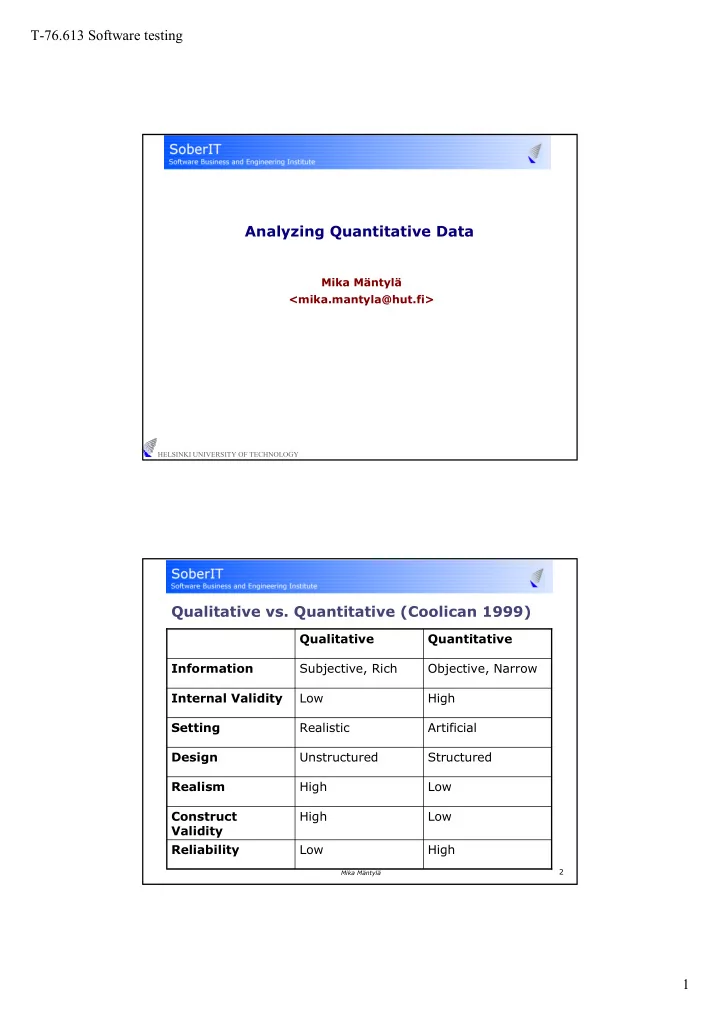
T-76.613 Software testing Analyzing Quantitative Data Mika Mntyl <mika.mantyla@hut.fi> HELSINKI UNIVERSITY OF TECHNOLOGY Qualitative vs. Quantitative (Coolican 1999) Qualitative Quantitative Information Subjective, Rich


  1. T-76.613 Software testing Analyzing Quantitative Data Mika Mäntylä <mika.mantyla@hut.fi> HELSINKI UNIVERSITY OF TECHNOLOGY Qualitative vs. Quantitative (Coolican 1999) Qualitative Quantitative Information Subjective, Rich Objective, Narrow Internal Validity Low High Setting Realistic Artificial Design Unstructured Structured Realism High Low Construct High Low Validity Reliability Low High 2 Mika Mäntylä 1

  2. T-76.613 Software testing Measurement Scales Why Ratio � � Determine the applicability of E.g.: Temperature K°, Length in � � statistical tests centimeters Arithmetic Operations: Nominal � � Multiplication & division E.g.: Gender � Rational zero and equivalent � Arithmetic Operations: Counting � ratios No numeric meaning � Ordinal or Interval? � Ordinal � Importance of listed activities in � E.g.: Movie ratings, Likert scale standard Likert scale (i.e. � data, Rankings completely agree, somewhat agree, neither agree or disagree, Arithmetic Operations: Size � somewhat agree, completely comparisons disagree) Intervals between scale values � Ordinal? are undefined � Distribute 100 point based on the � Interval � importance of activities E.g.: Temperature C°, IQ scores � Interval? � Arithmetic Operations: Addition & � Subtraction Intervals between scale values � are equal 3 Mika Mäntylä Distributions � Why � Determine the applicability of statistical tests � Normal Distribution � Assumed in most parametric tests � Most biological measure are have normal or lognormal distribution � Many psychological and educational test are fitted to normal distribution for research purposes � Likert scale (1-5) is not normally distributed � Too few options i.e. cannot answer 1.25 etc � Often the answers are skewed towards one end i.e. not mount shaped � Power Laws and Distributions (Pareto, Zipf) � Many phenomena follow power distribution � City sizes, wealth, word frequencies, earthquake magnitudes, sources of software failures, visits of websites 4 Mika Mäntylä 2

  3. T-76.613 Software testing Zipf’s Law – JDK 5 Mika Mäntylä Probability density functions (Wikibedia) � Normal, LogNormal, 6 Mika Mäntylä 3

  4. T-76.613 Software testing Differences between two groups � Is there a difference: � In development time between team using pair- programming and solo-programming � In credit card spending between people receiving promotions and not receiving promotions � In company sizes between software product companies and software companies � t-test is popular test for measuring a difference of single variable between two groups � Example: Credit card spending (SPSS) Independent Samples Test Equal variances assumed Levene's Test for Equality of Variances t-test for Equality of Means 95% Confidence Interval of the Difference Mean Std. Error F Sig. t df Sig. (2-tailed) Difference Difference Lower Upper $ spent during 7 Mika Mäntylä 1,190 ,276 -2,260 498 ,024 -71,11095 31,45914 -132,920 -9,30196 promotional period Differences between two groups - cont’d � Example: Software company sizes Group Statistics Std. Error Type N Mean Std. Deviation Mean Employees Software 529 57,7958 174,91927 7,60519 SoftwareProduct 471 91,3758 319,76937 14,73419 Independent Samples Test Levene's Test for Equality of Variances t-test for Equality of Means 95% Confidence Interval of the Difference Mean Std. Error F Sig. t df Sig. (2-tailed) Difference Difference Lower Upper Employees Equal variances 12,875 ,000 -2,090 998 ,037 -33,57995 16,06980 -65,11442 -2,04549 assumed Equal variances -2,025 708,999 ,043 -33,57995 16,58117 -66,13403 -1,02588 not assumed 8 Mika Mäntylä 4

  5. T-76.613 Software testing Differences between two groups - cont’d � Assumptions of t-test � Interval scale � Normal (or near normal) distribution � Both assumptions hold for credit card example data � What about software company sizes? 9 Mika Mäntylä Differences between two groups - cont’d � Mann-Whitney (or Wilcoxon-Mann-Whitney) test is non-parametric alternative to t-test � Software company sizes with non-parametric test Ranks Type N Mean Rank Sum of Ranks Employees Software 529 496,63 262715,50 SoftwareProduct 471 504,85 237784,50 Total 1000 a Test Statistics Employees Mann-Whitney U 122530,500 Wilcoxon W 262715,500 Z -,450 Asymp. Sig. (2-tailed) ,653 a. Grouping Variable: Type 10 Mika Mäntylä 5

  6. T-76.613 Software testing Correlation between two variables The degree to which the variables are related (i.e. co-vary) � http://noppa5.pc.helsinki.fi/koe/corr/cor7.html Parametric (Pearson) and non-parametric (Spearman, Kendall’s Tau) � � Pearson: Variables are interval scale, and (approximately) normally distributed � Spearman is more widely used and easier to compute than Tau. � Kendall’s Tau has better statistical properties than Spearman � “Results suggest that Kendalls tau(b) has many advantages over Pearsons and Spearmans r ; when applied to psychiatric data.“ (Arndt et al. 1999) Term “high correlation” has no strict boundaries � � 0.00 – 0.20: no correlation; 0.20 – 0.40: low correlation; 0.40 – 0.70: moderate correlation; 0.70 – 0.90: high correlation; 0.90 – 1.00: very high correlation; Significance (the chance of obtaining the result by change) of � correlation � Computed based correlation coefficient and sample size Correlation does not indicate causal relationships � 11 Mika Mäntylä More than two variables - Partial Correlation � Correlation can only tell the relation of two variables � What if there are several related variables � Partial Correlation (Parametric method) � Regression (Next Slide) � Partial Correlation Example: � Variables � T = study time; S = exam score; F = fear of the professor � Correlations � r(TS) = 0,2; r(TF) = 0,8; r(SF) =-0,4 r ( r r ) − ∗ r TS TF SF � Partial correlation from the equation: = TS F • 2 2 1 r 1 r − ∗ − � r(TS · F)=0,95 TF SF � Interpretation: Study time is highly correlated with test score when fear is removed / held constant 12 Mika Mäntylä 6

  7. T-76.613 Software testing Predicting Single Variable - Regression � Correlation indicates how well a line fits the data � Regression line is the “best line” � Minimizes the sum of squared distances from the line � y=b+mx � Regression example from SPSS 13 Mika Mäntylä 7

  8. T-76.613 Software testing Predicting Single Variable - Regression � Correlation indicates how well a line fits the data � Regression line is the “best line” � minimizes the sum of squared vertical distances from the line � y=b+mx � In this case the equation becomes � time = -1,955 + diameter * 3,457 � Regression is often used for prediction � Time estimate for polishing 15 inch object � -1,955 + 15*3,457 = 49,9 minutes � Strength of the regression line � R (0,700)–correlation coefficient � R^2 (0,490)–percentage of variation explained (co-variation) � Adjusted R^2 (0,482) – adjusted based on model complexity, more conservative than R^2 15 Mika Mäntylä Predicting Single Variable - Regression There is no reason to have only a single predictor � � Multiple Regression: y=b+mx1+nx2+ox3+px4 � Line that minimizes the distances from y in multidimensional space Common uses of multiple regression (other than prediction) � � Controlling a variable � Confounding effect of size (Emam et al 2001). “After controlling for size, none of the metrics we studied were associated with — fault-proneness anymore.” � Best combined predictors � Best combination of techniques to reduce defect rate: (MacCormack 2003) Early prototype, design review, regression-test — Others were also correlated, but they were not significant in the regression — model Several variations of regression exists � � Linear Regression, Logistic Regression, Categorical Regression, etc. � Find a regression that is suitable for your data Other more advanced techniques: Structural Equation Modeling � 16 Mika Mäntylä 8

  9. T-76.613 Software testing Weaknesses in linear models Look beyond the numbers ! � Four data sets with equal values (KQR 2005) � N=11; Avg X = 9,0; Avg Y=7,5; Regression line y=3+0,5x; r^2=0,67; I II 10 10 5 5 0 0 0 10 20 0 10 20 IV III 10 10 5 5 0 0 0 10 20 0 10 20 18 Mika Mäntylä 9

Download Presentation
Download Policy: The content available on the website is offered to you 'AS IS' for your personal information and use only. It cannot be commercialized, licensed, or distributed on other websites without prior consent from the author. To download a presentation, simply click this link. If you encounter any difficulties during the download process, it's possible that the publisher has removed the file from their server.

Recommend


More recommend