Symbol-table problem Symbol table T holding n records : record x - - PowerPoint PPT Presentation

CS 5633 Analysis of Algorithms 1 2/22/05

CS 5633 -- Spring 2005

Hashing

Carola Wenk Slides courtesy of Charles Leiserson with small changes by Carola Wenk

CS 5633 Analysis of Algorithms 2 2/22/05

Symbol-table problem

Symbol table T holding n records: key[x] key[x]

record

x

Other fields containing satellite data

Operations on T:

• INSERT(T, x)
• DELETE(T, x)
• SEARCH(T, k)

How should the data structure T be organized?

CS 5633 Analysis of Algorithms 3 2/22/05

Direct-access table

IDEA: Suppose that the set of keys is K ⊆ {0, 1, …, m–1}, and keys are distinct. Set up an array T[0 . . m–1]: T[k] = x if key[x] = k ∈ K ,

NIL

• therwise.

Then, operations take Θ(1) time. Problem: The range of keys can be large:

• 64-bit numbers (which represent

18,446,744,073,709,551,616 different keys),

• character strings (even larger!).

CS 5633 Analysis of Algorithms 4 2/22/05

As each key is inserted, h maps it to a slot of T.

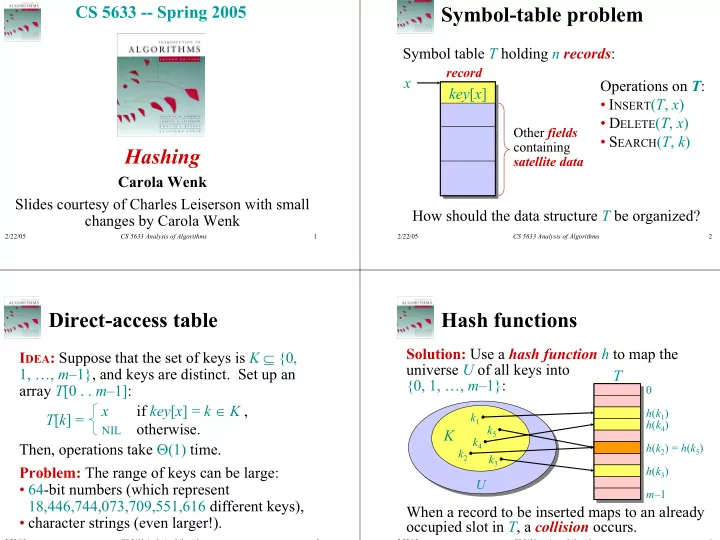
Hash functions

Solution: Use a hash function h to map the universe U of all keys into {0, 1, …, m–1}:

U

K

k1 k2 k3 k4 k5 m–1 h(k1) h(k4) h(k2) h(k3)

When a record to be inserted maps to an already

• ccupied slot in T, a collision occurs.

T

= h(k5)

CS 5633 Analysis of Algorithms 5 2/22/05

Resolving collisions by chaining

• Records in the same slot are linked into a list.

h(49) = h(86) = h(52) = i

T 49 49 86 86 52 52

i

CS 5633 Analysis of Algorithms 6 2/22/05

Analysis of chaining

We make the assumption of simple uniform hashing:

• Each key k ∈ K of keys is equally likely to

be hashed to any slot of table T, independent

• f where other keys are hashed.

Let n be the number of keys in the table, and let m be the number of slots. Define the load factor of T to be α = n/m = average number of keys per slot.

CS 5633 Analysis of Algorithms 7 2/22/05

Search cost

Expected time to search for a record with a given key = Θ(1 + α).

apply hash function and access slot search the list

Expected search time = Θ(1) if α = O(1),

• r equivalently, if n = O(m).

CS 5633 Analysis of Algorithms 8 2/22/05

Choosing a hash function

The assumption of simple uniform hashing is hard to guarantee, but several common techniques tend to work well in practice as long as their deficiencies can be avoided. Desirata:

• A good hash function should distribute the

keys uniformly into the slots of the table.

• Regularity in the key distribution should

not affect this uniformity.

CS 5633 Analysis of Algorithms 9 2/22/05

h(k)

Division method

Assume all keys are integers, and define h(k) = k mod m. Extreme deficiency: If m = 2r, then the hash doesn’t even depend on all the bits of k:

• If k = 10110001110110102 and r = 6, then

h(k) = 0110102 . Deficiency: Don’t pick an m that has a small divisor d. A preponderance of keys that are congruent modulo d can adversely affect uniformity.

CS 5633 Analysis of Algorithms 10 2/22/05

Division method (continued)

h(k) = k mod m. Pick m to be a prime not too close to a power

• f 2 or 10 and not otherwise used prominently

in the computing environment. Annoyance:

• Sometimes, making the table size a prime is

inconvenient.

CS 5633 Analysis of Algorithms 11 2/22/05

Resolving collisions by open addressing

No storage is used outside of the hash table itself.

• Insertion systematically probes the table until an

empty slot is found.

• The hash function depends on both the key and

probe number: h : U × {0, 1, …, m–1} → {0, 1, …, m–1}.

• The probe sequence 〈h(k,0), h(k,1), …, h(k,m–1)〉

should be a permutation of {0, 1, …, m–1}.

• The table may fill up, and deletion is difficult (but

not impossible).

CS 5633 Analysis of Algorithms 12 2/22/05

204 204

Example of open addressing

Insert key k = 496:

• 0. Probe h(496,0)

586 133 481

T

m–1

collision

CS 5633 Analysis of Algorithms 13 2/22/05

Example of open addressing

Insert key k = 496:

• 0. Probe h(496,0)

586 133 204 481

T

m–1

• 1. Probe h(496,1)

collision

586

CS 5633 Analysis of Algorithms 14 2/22/05

Example of open addressing

Insert key k = 496:

• 0. Probe h(496,0)

586 133 204 481

T

m–1

• 1. Probe h(496,1)

insertion

496

• 2. Probe h(496,2)

CS 5633 Analysis of Algorithms 15 2/22/05

Example of open addressing

Search for key k = 496:

• 0. Probe h(496,0)

586 133 204 481

T

m–1

• 1. Probe h(496,1)

496

• 2. Probe h(496,2)

Search uses the same probe sequence, terminating suc- cessfully if it finds the key and unsuccessfully if it encounters an empty slot.

CS 5633 Analysis of Algorithms 16 2/22/05

Probing strategies

Linear probing: Given an ordinary hash function h′(k), linear probing uses the hash function h(k,i) = (h′(k) + i) mod m. This method, though simple, suffers from primary clustering, where long runs of occupied slots build up, increasing the average search time. Moreover, the long runs of occupied slots tend to get longer.

CS 5633 Analysis of Algorithms 17 2/22/05

Probing strategies

Double hashing Given two ordinary hash functions h1(k) and h2(k), double hashing uses the hash function h(k,i) = (h1(k) + i⋅h2(k)) mod m. This method generally produces excellent results, but h2(k) must be relatively prime to m. One way is to make m a power of 2 and design h2(k) to produce only odd numbers.

CS 5633 Analysis of Algorithms 18 2/22/05

Analysis of open addressing

We make the assumption of uniform hashing:

• Each key is equally likely to have any one of

the m! permutations as its probe sequence.

• Theorem. Given an open-addressed hash

table with load factor α = n/m < 1, the expected number of probes in an unsuccessful search is at most 1/(1–α).

CS 5633 Analysis of Algorithms 19 2/22/05

Proof of the theorem

Proof.

• At least one probe is always necessary.
• With probability n/m, the first probe hits an
• ccupied slot, and a second probe is necessary.
• With probability (n–1)/(m–1), the second probe

hits an occupied slot, and a third probe is necessary.

• With probability (n–2)/(m–2), the third probe

hits an occupied slot, etc. Observe that α = < − − m n i m i n for i = 1, 2, …, n.

CS 5633 Analysis of Algorithms 20 2/22/05

Proof (continued)

Therefore, the expected number of probes is                         + − + − − + − − + + L L 1 1 1 2 2 1 1 1 1 1 n m m n m n m n

( ) ( ) ( ) ( )

α α α α α α α α α − = = + + + + ≤ + + + + ≤

∑

∞ =

1 1 1 1 1 1 1

3 2 i i

L L L . The textbook has a more rigorous proof.

CS 5633 Analysis of Algorithms 21 2/22/05

Implications of the theorem

• If α is constant, then accessing an open-

addressed hash table takes constant time.

• If the table is half full, then the expected

number of probes is 1/(1–0.5) = 2.

• If the table is 90% full, then the expected

number of probes is 1/(1–0.9) = 10.