Switching and Forwarding Outline Store-and-Forward Switches - - PDF document

1

1

Switching and Forwarding

Outline

Store-and-Forward Switches Bridges and Extended LANs Cell Switching Segmentation and Reassembly

2

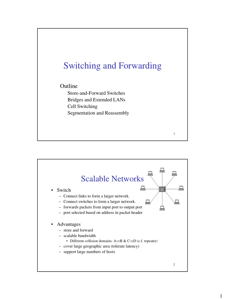
Scalable Networks

• Switch

– Connect links to form a larger network. – Connect switches to form a larger network. – forwards packets from input port to output port – port selected based on address in packet header

• Advantages

– store and forward – scalable bandwidth

• Different collision domains: A⇒B & C⇒D (c.f. repeater)

– cover large geographic area (tolerate latency) – support large numbers of hosts

2

3

Source Routing

1 3 2 1 3 2 1 3 2 1 3 2 3 0 1 3 0 1 3 0 1 Switch 3 Host B Switch 2 Host A Switch 1

A places port numbers along the path in packet headers. B sends in the reverse order. Header is long The sender must knows the topology

4

Virtual Circuit Switching

• Explicit connection setup (and tear-down) phase

– Sometimes called connection-oriented model

• Subsequence packets follow same circuit
• Each switch maintains a VC table
• Virtual Circuit

– Virtual Circuit Identifier (VCI)

• Uniquely identify a VC at a switch

– Permanent VC (PVC) configured by administrator – Switched VC (SVC) setup by hosts

• signaling

3

5

Virtual Circuit Tables

Switch In If In VCI Out If Out VCI 1 2 5 1 11 … … … 2 3 11 2 7 … … … 3 7 1 4 … … …

1 2 3 1 2 3 1 3 1 2 3 Host A Host B Switch 3 Switch 2 Switch 1 7 5 4 11 2

VCI locally unique, to avoid the problem of providing a globally unique VCI

6

Virtual Circuit Model

• Typically wait full RTT for connection setup before sending

first data packet.

• While the connection request contains the full address for

destination, each subsequent data packet contains only a small identifier

– make the per-packet header overhead small.

• If a switch or a link in a connection fails, the connection is

broken and a new one needs to be established.

• Connection setup provides an opportunity to reserve

resources for QoS.

– Admission control (Analogy: phone call)

4

7

Establishing VC (1)

• Node A sends a Connection request Message to

Node B.

– Initially the message is sent across a direct link to Switch 1; The message contains the address of both A and B

• Switch 1 establishes a new entry in its Virtual

Circuit Table

– Incoming interface – Incoming VCI

• Each switch in turn selects a unique VCI for the incoming link

– Outgoing interface

• The switch must therefore know the network topology

– Outgoing VCI

• The outgoing VCI is in turn chosen by the next switch

8

Establishing VC (2)

• When Node B receives the connection request

– It then returns an acceptance message ( or possibly a rejection) to Node A – This acceptance message includes the VCI it has selected

• The first switch on the return route can now fill in

the outgoing VCI in its Virtual Circuit Table

• This switch in turn substitutes the VCI it has

chosen for its incoming link and forwards the acceptance message to the previous switch

5

9

Datagram Switching

• No connection setup phase

– Sometimes called connectionless model

• Each packet forwarded independently
• Each switch maintains a forwarding (routing) table

– Eg. Switch 1

1 3 2 1 3 2 1 3 2 Switch 3 Host B Switch 2 Host A Switch 1 Host C Host D Host E Host F Host G Host H

Address Port A 2 C 3 F 1 G 1 … …

10

Datagram Model

• There is no round trip delay waiting for connection setup; a

host can send data as soon as it is ready.

• Source host has no way of knowing if the network is

capable of delivering a packet or if the destination host is even up.

– No QoS

• Since packets are treated independently, it is possible to

route around link and node failures.

• Since every packet must carry the full address of the

destination, the overhead per packet is higher than for the connection-oriented model.

6

11

Bridges and Extended LANs

• Connect two or more LANs with a bridge

– LANs have physical limitations – Not repeaters – Different collision domains: Store and forward strategy

A Bridge B C X Y Z Port 1 Port 2 12

• Do not forward to all the other ports (broadcast)

when unnecessary

• Maintain forwarding table

Host Port A 1 B 1 C 1 X 2 Y 2 Z 2

• Learn table entries based on source address
• Table is an optimization; need not be complete
• Always forward broadcast frames

Learning Bridges

A Bridge B C X Y Z Port 1 Port 2

7

13

Broadcast and Multicast

• Switches forward all broadcast/multicast

frames

• Multicast: let the hosts decide whether to

accept the frame

– Configure the adaptor – Current practice

14

Spanning Tree Algorithm

• Broadcast: loop for ever

– Even unicast messages with unlearned destination will be broadcasted. – Loops may span many links!

• Shortest Path Tree:
• Bridges run a distributed spanning tree algorithm

– Bridges do not have the global topology – Select which port to be “logically” pruned in the tree – Dynamic reconfigure when some bridges fail.

(a) (b)

8

15

Extended LAN with Loops

A C E D B K F H J G I B5 B2 B3 B7 B4 B1 B6 16

Algorithm Overview

• Each bridge or LAN is a node in the graph.
• Each bridge has unique id (e.g., B1, B2, B3). Select

bridge with smallest id as root

• Active Ports of a Bridge

– 1 Root port: Who is my parent?

• Shortest path to the root.

– Designated Ports: Who are my children?

• Among all bridges attached to a LAN, select the one closest to root

as designated bridge (use id to break ties) for the LAN. The corresponding port is a designated port on the bridge

• All ports of a root bridge are designated ports

– Prune all other ports.

9

17

Algorithm Details

• Bridges exchange configuration messages (bridge protocol

data units BPDU)

– id for what the sending bridge believes to be root bridge – distance (hops) from sending bridge to root bridge – id for bridge sending the message – The port id of the sending bridge

• In case two bridges share two segments!
• Each bridge records current best configuration message for

each port

– If root id is smaller, or the path hops is smaller – Otherwise, if the id or port id of the sending bridge is smaller

18

Algorithm Detail (cont)

• Discard BPDU if it is not better than the best configuration

for the receiving port

– Stateful: No broadcast storms!

• Otherwise,

– Update configuration for the receiving port – Update the state of the switch – Forward the BPDU to all the other ports, with distance +1 and new sending bridge id

• Self-Configuration

– Initially, each bridge believes it is the root – When learn not root, stop generating its own messages – Root continues to periodically send config messages – If any bridge does not receive config message after a period of time, it starts generating config messages claiming to be the root

10

19

Limitations of Bridges

• Do not scale

– spanning tree algorithm does not scale – broadcast does not scale

• Do not accommodate heterogeneity of networks

20

Cell Switching (ATM)

• Connection-oriented packet-switched network
• Used in both WAN and LAN settings
• Packets are called cells

– 5-byte header + 48-byte payload

• Commonly transmitted over SONET

– other physical layers possible

11

21

Variable vs Fixed-Length Packets

• Fixed-Length Easier to Switch in Hardware

– Simpler with the knowledge of packet length – Easier to enable parallelism

• No Optimal Length for Fixed-Length Cells

– if small: high header-to-data overhead – if large: low bit utilization for small messages

• Padding: the number of valid bytes is indicated in the header

22

Big vs Small Packets

• Small Improves Queue behavior

– finer-grained preemption point for scheduling link

• maximum packet = 4KB
• link speed = 100Mbps
• transmission time = 4096 x 8/100 = 327.68us
• high priority packet may sit in the queue 327.68us
• in contrast, 53 x 8/100 = 4.24us for ATM

– Smaller queues

• two 4KB packets arrive at same time
• link idle for 327.68us while both arrive

– wait for the whole packet

• at end of 327.68us, still have 8KB to transmit
• in contrast, can transmit first cell after 4.24us
• at end of 327.68us, just over 4KB left in queue

12

23

Big vs Small (cont)

• Small Improves Latency (for voice)

– voice digitally encoded at 64KBps (8-bit samples at 8KHz) – need full cell’s worth of samples before sending cell – example: 1000-byte cells implies 125ms per cell (too long) – smaller latency implies no need for echo cancellers

• ATM Compromise: 48 bytes