Summary: Wavelet Scattering Net x ( u ) | x 1 | ( u ) - - PowerPoint PPT Presentation

Summary: Wavelet Scattering Net

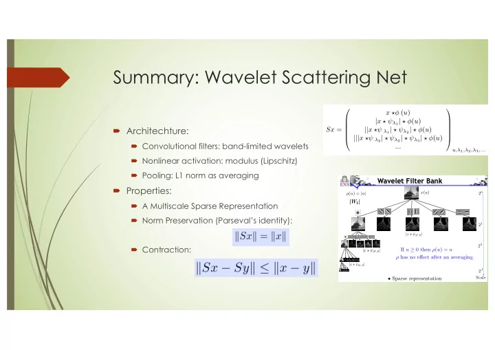
´ Architechture:

´ Convolutional filters: band-limited wavelets ´ Nonlinear activation: modulus (Lipschitz) ´ Pooling: L1 norm as averaging

´ Properties:

´ A Multiscale Sparse Representation ´ Norm Preservation (Parseval’s identity): ´ Contraction:

Sx =       x ⇤ (u) |x ⇤ ⇥λ1| ⇤ (u) ||x ⇤⇥ λ1| ⇤ ⇥λ2| ⇤ (u) |||x ⇤⇥ λ2| ⇤ ⇥λ2| ⇤ ⇥λ3| ⇤ (u) ...      

u,λ1,λ2,λ3,...

k k )) k Sx

is

20 22 2J |x ? 22,θ|

|W1|

Scale 21

|x ? 21,θ|

|W1|

Wavelet Filter Bank

x(u) ρ(α) = |α|

• Sparse representation

|x ? 2j,θ|

If u ≥ 0 then ρ(u) = u ρ has no effect after an averaging.

Invariants/Stability of Scattering Net

´ Translation Invariance: ´ Stable Small Deformations:

• The average |x ? λ1| ? (t) is invariant to small translations

relatively to the support of φ. lim

φ→1 |x ? λ1| ? (t) =

Z |x ? λ1(u)| du = kx ? λ1k1

Feature Extraction

LeCun et. al.

Classification Errors Joan Bruna

Digit Classification: MNIST

SJx y = f(x) x Supervised Linear classifier

Invariants to specific deformations Separates different patterns Invariants to translations Linearises small deformations No learning

Training size

• Conv. Net.

Scattering 50000 0.4% 0.4%

Other Invariants? General Convolutional Neural Networks?

UIUC database: 25 classes Scattering classification errors Training

• Scat. Translation

20 20 %

Rotation and Scaling Invariance

Laurent Sifre

x(u) x1(u, k1) x2(u, k2) xJ(u, kJ) k1 k2

Deep Convolutional Trees

ρL1 ρLJ xj = ρ Lj xj−1

classification

Lj is composed of convolutions and subs samplings: xj(u, kj) = ⇢ ⇣ xj−1(·, k) ? hkj,k(u) ⌘ No channel communication: what limitations ?

x(u) x1(u, k1) x2(u, k2) xJ(u, kJ) k1 k2

Deep Convolutional Networks

ρL1 ρLJ xj = ρ Lj xj−1 xj(u, kj) = ⇢ ⇣ X

k

xj−1(·, k) ? hkj,k(u) ⌘

sum across channels

classification

• Lj is a linear combination of convolutions and subsampling:

What is the role of channel connections ? Linearize other symmetries beyond translations.

Rotation Invariance

2J

|x ? 22,θ| |x ? 23,θ| Scale

|x ? 21,θ|

|W1|

x ? J

θ

• Channel connections linearize other symmetries.
• Invariance to rotations are computed by convolutions

along the rotation variable θ with wavelet filters. ⇒ invariance to rigid mouvements.

Xj ~ φ(r, t)

|Xj ~ ψλ2(r, t)|

• Averaging on G:

X ~ φ(g) = Z

G

X(g0) φ(g

01g) dg0

• Wavelet transform on G:

W2X = ✓ X ~ φ(g) X ~ ψλ2(g) ◆

λ2,g

. |W1| |W2|

Wavelet Transform on a Group

x x ? (t) |x ? 2jr(t)| translation roto-translation = Xj(r, t) (r, t) . x(u) = x(r−1(u − t))

• Roto-translation group G = {g = (r, t) ∈ SO(2) × R2}

Laurent Sifre

X ~ φ(2j, r, t)

|X ~ ψλ2(2j, r, t)|

• Averaging on G:

X ~ φ(g) = Z

G

X(g0) φ(g

01g) dg0

• Wavelet transform on G:

W2X = ✓ X ~ φ(g) X ~ ψλ2(g) ◆

λ2,g

. |W1| |W2|

Wavelet Transform on a Group

x x ? (t) |x ? 2jr(t)| translation

scalo-roto-translation = X(2j, r, t)

+ renormalization

(r, t) . x(u) = x(r−1(u − t))

• Roto-translation group G = {g = (r, t) ∈ SO(2) × R2}

Laurent Sifre

UIUC database: 25 classes Scattering classification errors Training Translation Transl + Rotation + Scaling 20 20 % 2% 0.6%

Rotation and Scaling Invariance

Laurent Sifre

Wiatowski-Bolcskei’15

´ Scattering Net by Mallat et al. so far

´ Wavelet Linear filter ´ Nonlinear activation by modulus ´ Average pooling

´ Generalization by Wiatowski-Bolcskei’15

´ Filters as frames ´ Lipschitz continuous Nonlinearities ´ General Pooling: Max/Average/Nonlinear, etc.

Generalization of Wiatowski-Bolcskei’15

Scattering networks ([Mallat, 2012], [Wiatowski and HB, 2015])

feature map feature vector Φ(f)

f |f ∗ gλ(k)

1 |

· ∗ χ2 ||f ∗ gλ(k)

1 | ∗ gλ(l) 2 |

· ∗ χ3 |f ∗ gλ(p)

1 |

· ∗ χ2 ||f ∗ gλ(p)

1 | ∗ gλ(r) 2 |

· ∗ χ3 · ∗ χ1

General scattering networks guarantee [Wiatowski & HB, 2015]

• (vertical) translation invariance
• small deformation sensitivity

essentially irrespective of filters, non-linearities, and poolings!

Wavelet basis -> filter frame

´

Building blocks

Basic operations in the n-th network layer f . . . gλ(r)

n

non-lin. pool. gλ(k)

n

non-lin. pool. Filters: Semi-discrete frame Ψn := {χn} [ {gλn}λn∈Λn Ankfk2

2  kf ⇤ χnk2 2 +

X

λn∈Λn

kf ⇤ gλnk2  Bnkfk2

2,

8f 2 L2(Rd) e.g.: Structured filters

Frames: random or learned filters

Building blocks

Basic operations in the n-th network layer f . . . gλ(r)

n

non-lin. pool. gλ(k)

n

non-lin. pool. Filters: Semi-discrete frame Ψn := {χn} [ {gλn}λn∈Λn Ankfk2

2  kf ⇤ χnk2 2 +

X

λn∈Λn

kf ⇤ gλnk2  Bnkfk2

2,

8f 2 L2(Rd) e.g.: Learned filters

Building blocks

Basic operations in the n-th network layer f . . . gλ(r)

n

non-lin. pool. gλ(k)

n

non-lin. pool. Filters: Semi-discrete frame Ψn := {χn} [ {gλn}λn∈Λn Ankfk2

2  kf ⇤ χnk2 2 +

X

λn∈Λn

kf ⇤ gλnk2  Bnkfk2

2,

8f 2 L2(Rd) e.g.: Unstructured filters

Nonlinear activations

Building blocks

Basic operations in the n-th network layer f . . . gλ(r)

n

non-lin. pool. gλ(k)

n

non-lin. pool. Non-linearities: Point-wise and Lipschitz-continuous kMn(f) Mn(h)k2  Lnkf hk2, 8 f, h 2 L2(Rd) ) Satisfied by virtually all non-linearities used in the deep learning literature! ReLU: Ln = 1; modulus: Ln = 1; logistic sigmoid: Ln = 1

4; ...

Pooling

Building blocks

Basic operations in the n-th network layer f . . . gλ(r)

n

non-lin. pool. gλ(k)

n

non-lin. pool. Pooling: In continuous-time according to f 7! Sd/2

n

Pn(f)(Sn·), where Sn 1 is the pooling factor and Pn : L2(Rd) ! L2(Rd) is Rn-Lipschitz-continuous

) Emulates most poolings used in the deep learning literature! e.g.: Pooling by sub-sampling Pn(f) = f with Rn = 1 e.g.: Pooling by averaging Pn(f) = f ⇤ φn with Rn = kφnk1

Vertical translation invariance

Theorem (Wiatowski and HB, 2015) Assume that the filters, non-linearities, and poolings satisfy Bn  min{1, L−2

n R−2 n },

8 n 2 N. Let the pooling factors be Sn 1, n 2 N. Then, |||Φn(Ttf) Φn(f)||| = O ✓ ktk S1 . . . Sn ◆ , for all f 2 L2(Rd), t 2 Rd, n 2 N. The condition Bn  min{1, L−2

n R−2 n },

8 n 2 N, is easily satisfied by normalizing the filters {gλn}λn∈Λn.

Vertical translation invariance

Theorem (Wiatowski and HB, 2015) Assume that the filters, non-linearities, and poolings satisfy Bn  min{1, L−2

n R−2 n },

8 n 2 N. Let the pooling factors be Sn 1, n 2 N. Then, |||Φn(Ttf) Φn(f)||| = O ✓ ktk S1 . . . Sn ◆ , for all f 2 L2(Rd), t 2 Rd, n 2 N. ) Features become more invariant with increasing network depth!

Vertical translation invariance

Theorem (Wiatowski and HB, 2015) Assume that the filters, non-linearities, and poolings satisfy Bn  min{1, L−2

n R−2 n },

8 n 2 N. Let the pooling factors be Sn 1, n 2 N. Then, |||Φn(Ttf) Φn(f)||| = O ✓ ktk S1 . . . Sn ◆ , for all f 2 L2(Rd), t 2 Rd, n 2 N. Full translation invariance: If lim

n→∞ S1 · S2 · . . . · Sn = 1, then

lim

n→∞ |||Φn(Ttf) Φn(f)||| = 0

Philosophy behind invariance results

Mallat’s “horizontal” translation invariance [Mallat, 2012]: lim

J→∞ |||ΦW (Ttf) − ΦW (f)||| = 0,

∀f ∈ L2(Rd), ∀t ∈ Rd

• features become invariant in every network layer, but needs

J → ∞

• applies to wavelet transform and modulus non-linearity without

pooling “Vertical” translation invariance: lim

n→∞ |||Φn(Ttf) − Φn(f)||| = 0,

∀f ∈ L2(Rd), ∀t ∈ Rd

• features become more invariant with increasing network depth
• applies to general filters, general non-linearities, and general

poolings

Non-linear deformations

Non-linear deformation (Fτf)(x) = f(x − τ(x)), where τ : Rd → Rd For “small” τ:

Non-linear deformations

Non-linear deformation (Fτf)(x) = f(x − τ(x)), where τ : Rd → Rd For “large” τ:

Deformation sensitivity for signal classes

Consider (Fτf)(x) = f(x − τ(x)) = f(x − e−x2)

x f1(x), (Fτf1)(x) x f2(x), (Fτf2)(x)

For given τ the amount of deformation induced can depend drastically on f ∈ L2(Rd)

Wiatowski-Bolcskei’15 Deformation Stability Bounds

Philosophy behind deformation stability/sensitivity bounds

Mallat’s deformation stability bound [Mallat, 2012]: |||ΦW (Fτf)ΦW (f)|||  C

• 2−Jkτk∞ +JkDτk∞ +kD2τk∞
• kfkW ,

for all f 2 HW ✓ L2(Rd)

• The signal class HW and the corresponding norm k · kW depend
• n the mother wavelet (and hence the network)

Our deformation sensitivity bound: |||Φ(Fτf) Φ(f)|||  CCkτkα

∞,

8f 2 C ✓ L2(Rd)

• The signal class C (band-limited functions, cartoon functions, or

Lipschitz functions) is independent of the network

Philosophy behind deformation stability/sensitivity bounds

Mallat’s deformation stability bound [Mallat, 2012]: |||ΦW (Fτf)ΦW (f)|||  C

• 2−Jkτk∞ +JkDτk∞ +kD2τk∞
• kfkW ,

for all f 2 HW ✓ L2(Rd)

• Signal class description complexity implicit via norm k · kW

Our deformation sensitivity bound: |||Φ(Fτf) Φ(f)|||  CCkτkα

∞,

8f 2 C ✓ L2(Rd)

• Signal class description complexity explicit via CC
• L-band-limited functions: CC = O(L)
• cartoon functions of size K: CC = O(K3/2)
• M-Lipschitz functions CC = O(M)

Wiatowski-Bolcskei’15 Deformation Stability Bounds

Philosophy behind deformation stability/sensitivity bounds

Mallat’s deformation stability bound [Mallat, 2012]: |||ΦW (Fτf)ΦW (f)|||  C

• 2−Jkτk∞ +JkDτk∞ +kD2τk∞
• kfkW ,

for all f 2 HW ✓ L2(Rd)

• The bound depends explicitly on higher order derivatives of τ

Our deformation sensitivity bound: |||Φ(Fτf) Φ(f)|||  CCkτkα

∞,

8f 2 C ✓ L2(Rd)

• The bound implicitly depends on derivative of τ via the

condition kDτk∞ 

1 2d

Philosophy behind deformation stability/sensitivity bounds

Mallat’s deformation stability bound [Mallat, 2012]: |||ΦW (Fτf)ΦW (f)|||  C

• 2−Jkτk∞ +JkDτk∞ +kD2τk∞
• kfkW ,

for all f 2 HW ✓ L2(Rd)

• The bound is coupled to horizontal translation invariance

lim

J→∞ |||ΦW (Ttf) ΦW (f)||| = 0,

8f 2 L2(Rd), 8t 2 Rd Our deformation sensitivity bound: |||Φ(Fτf) Φ(f)|||  CCkτkα

∞,

8f 2 C ✓ L2(Rd)

• The bound is decoupled from vertical translation invariance

lim

n→∞ |||Φn(Ttf) Φn(f)||| = 0,

8f 2 L2(Rd), 8t 2 Rd

x(u) x1(u, k1) x2(u, k2) xJ(u, kJ) k1 k2

Deep Convolutional Networks

ρL1 ρLJ

classification

• The convolution network operators have many roles:

– Linearize non-linear transformations (symmetries) – Reduce dimension with projections – Memory storage of « characteristic » structures

• Difficult to separate these roles when analyzing learned networks

Lj

x(u) x1(u, k1) x2(u, k2) xJ(u, kJ) k1 k2

Open Problems

ρL1 ρLJ

classification

• Can we recover symmetry groups from the matrices Lj ?
• What kind of groups ?
• Can we characterise the regularity of f(x) from these groups ?
• Can we define classes of high-dimensional « regular » functions

that are well approximated by deep neural networks ?

• Can we get approximation theorems giving errors depending on

number of training exemples, with a fast decay ?