
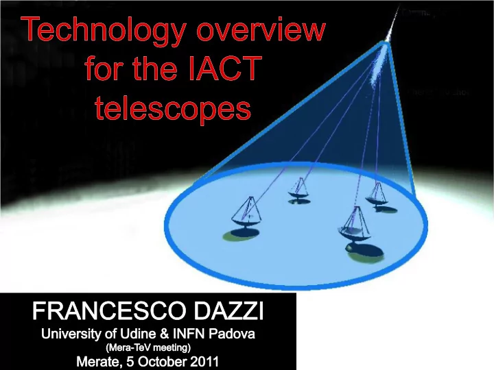
SLIDE 1
Summary Radiation observed Primary gamma ray Extended air - - PowerPoint PPT Presentation
Summary Radiation observed Primary gamma ray Extended air shower Cherenkov light & NSB Detector features IACT telescopes Reflective surface Light sensors Electronic chain Amplification
2
3
Image combines optical data from Hubble (in red) and X-ray images from Chandra (in blue).
Charged particle
4
v c n v c n
5
Particle shower Gamma-ray
~ 120 m
Max shower development
~ 10 km Detection of Detection of TeV gamma TeV gamma rays rays using Cherenkov using Cherenkov Telescopes Telescopes
~ 1o
6
Below 300 nm absorbed by ozone
Above 600÷700 nm dominated by LONS
LONS: diffuse light due to integrated starlight, air-glow & diffuse galactic light
NSB due to bright stars (LONS) = (1.75 ± 0.4) 1012 ph/m2 srs
IN THE CHERENKOV RANGE: 300-600nm
Bialkali PMT
EMISSION SPECTRUM OF LONS @ LA PALMA
EMISSION WATER HYDROXIDE ION EMISSION
REGION OF INTEREST
SIGNAL NOISE
7
input).
Trigger hardware input ~ 1 MHz
Trigger hardware output ~ 200 Hz (only accidental events and muons rejected)
γ rate after software analysis ~ 3 γ/min => 0,05 Hz (hadrons rejection)
S/N ~ 510-8 (1 good event every 20 millions)
400 m GROUND LIGHT DENSITY
Density < 10 photon/m2 at 100 GeV
CHERENKOV DENSITY
8
guarantee high rejection rate of noise and bad events
9
collected NSB photons.
(τgamma) => isochronous mirrors and electronics and fast trigger.
than the angular size of the shower (Ωshower) => small pixels.
gamma shower
NSB
NSB
NSB
10
VERITAS HESS MAGIC
11
Performances H.E.S.S. MAGIC VERITAS Sensitivity 0.7% 50h 0.9% 50h 0.7% 50h Trigger threshold 100 GeV 25 GeV 75 GeV Energy resolution 15% 15% 10-15% Angular resolution 0.06° 0.09° 0.03° Technical features H.E.S.S. MAGIC VERITAS Altitude 1800 m 2225 m 1275 m Telescope number 4 2 2 Reflector diameter 12 m 17 m 10 m Reflector genre Davies-Cotton Parabolic Davies-Cotton Focal distance 15 m 17 m 12 m Reflective area 107 m2 236 m2 106 m2 Mirrors technology Glass Al & glass Glass Number pixels 960 576 - 1039 499 Camera FoV 5° 3.5° 3.5° Light sensors kind PMT PMT PMT Light sensors QE 15% 20-30% 15-20% Complete rotation 3 min 40 s 3-4 min Readout 1 GS/s 2 GS/s 0.5 GS/s
0.10° 0.25° 0.15° Low energy threshold and high angular resolution Cost limitation & reduction of the channels number PIXEL SIZE 20m 5m 10m Low energy threshold & calibration with satellites Cost limitation & potential upgrade with high QE sensors DISH DIAMETER 5.0° 2.5° 3.5° Reduction images truncation and nice
extended sources Cost limitation & potential use of smaller pixels FoV f/1.5 f/0.7 f/1.2 Reduction aberrations Cost limitation & potential use of heavy camera OPTICAL SYSTEM
12
MIRROR SUPPORT PARABOLIC OR DAVIES-COTTON STRUCTURE CAMERA POSITION
~ 22 cm => 750 ps
13
MAGIC HESS VERITAS
14
MAGIC CASE
VERITAS HESS
It’s a well-known technology at relative low cost.
Unfortunately it is mature and so only small improvements are possible.
Low PDE between 20÷30%.
High PDE ~ 45% (QE: 50÷55%).
Better photon resolution than PMT.
Very expensive.
Low gain and high voltage.
Extremely high PDE between 60÷90%.
The best photon resolution.
Innovative and promising product.
Low voltage.
High dark current.
Not negligible crosstalk.
Small active area.
Low dynamic range
15
16
MAGIC HESS 22% 23% VERITAS
PDE (Photo Detection Efficiency).
Electric field between cathode & anode.
Dynodes gain.
Equal electrical answer, when PMTs are hit by the same light.
17 PDE
# photons => # phe
ELECTRIC FIELD
E electrons speed (Fixed active load preferred)
DYNODES GAIN
Gain charge
Low E => wide signal High E => tight signal
≠ SHAPE ≠ DELAY
Low Gain => small area High Gain => great area
≠ CHARGE
amplitude & width).
Get the same charge.
Fix the threshold in terms of photoelectrons and not in volts.
Minimize the skew between channels.
18
≠ SHAPE BUT SAME Q DT_1 DT_2
Amplitude_1 Amplitude_2 Width_1 Width_2
Delay_1 Delay_2 SAME NUMBER OF PHEs, BUT DIFFERENT ELECTRICAL SIGNAL: EQUALIZATION MANDATORY!!!
19
FRONT END electronics Local Trigger Readout - DAQ Stereo Trigger STORAGE FRONT END electronics Local Trigger Readout - DAQ STORAGE FRONT END electronics Local Trigger Readout - DAQ FRONT END electronics Local Trigger Readout - DAQ
20
21
afterpulses), preventing DAQ saturation.
L0: accept signals higher then an adjustable thresholds.
L1: fast coincidence (some nanoseconds) between neighbour PMTs (2-3-4-5 NN logic).
L2: enhanced topologic selection made with tree structured lookup table system and apply a prescaler factor.
L3: stereoscopic coincidence (100ns) between telescopes.
L1: CDF discriminator for each pixel at 4.2phe.
L2: 3 adjacent pixels exceed the threshold in 10ns.
L3: stereoscopic coincidence between telescopes.
L1: single pixel threshold at 4phe for 1.5ns.
L2: coincidence of 3 pixels in a sector of 64 pixels.
L3: stereoscopic coincidence (80ns) between at least 2 telescopes.
OK NO
TH t V
An on fly hardware trigger is mandatory, because the maximum DAQ rate is ~ 1KHz!
V (a.u.) t (a.u.) 22
to trigger, because images of low energy showers extend over many pixels. 19 pixels versus 4 close compact.
signal signal NSB Threshold (digital) Threshold (analog)
23
proper thresholds and new pixels are changed.
High thresholds Normal thresholds
24
Based on the analogue ring DRS chip (2GS/s), with a memory depth of 512ns
Commercial 8 bits FADC (0.5GS/s) with a memory depth of 64 s
Based on analogue ring sampler ARS0 circuit (1GS/s).
25
test instruments (TI), in order to improve its precision.
Mirror’s focusing
Mirror’s reflectivity
Dead pixels
Flat-fielding charge
Thresholds using IPRscan (Individual Pixel Rate scan) NSB (Night Sky Background)
Thresholds using IPRscan calibration laser
Delays synchronization
Effective gate equalization
Domino calibration run
Calibration & pedestal run
26
Raw data Time and gain corrected data
PMT
Transmitter
Optical Fibre
Receiver
Synchronization control
Trigger LT1 Trigger LT2 FADC
27
HESS
DRS input (mV) DRS output (FADC counts)
MAGIC
28
Temperature
Stars in the FoV [ Q ~ √phe]
Moon
Atmospherical conditions: clouds, humidity, calima, etc…
Electronic noise
Electronic fluctuations: FADC baseline, VCSEL stability
Interleaved calibration runs => conversion factors
Interleaved pedestal runs (It is the FADC output when the input is zero)
29
euro).
30
31
Weak light emitted by atoms in the upper atmosphere, due to UV radiation excitation.
Very faint light caused by sunlight scattered by space dust in the zodiacal cloud.
Light due to starlight reflected and scattered by interstellar dust near the galactic plane.
Light due to starlight reflected and scattered by interstellar dust.
32
Signal #1
(Reference)
Signal #2
(Minimum delay)
Signal #2
(Maximum delay)
GATE
(Overlap zone)
33
Raw data Time and gain corrected data
Signal
34
HESS VERITAS