Summary of part I: prediction and RL Prediction is important for - - PowerPoint PPT Presentation

Summary of part I: prediction and RL

Prediction is important for action selection

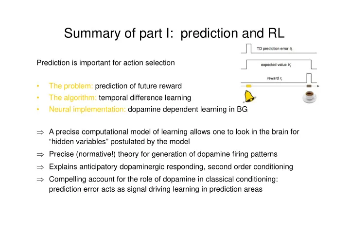
• The problem: prediction of future reward
• The algorithm: temporal difference learning
• Neural implementation: dopamine dependent learning in BG

⇒ A precise computational model of learning allows one to look in the brain for “hidden variables” postulated by the model ⇒ Precise (normative!) theory for generation of dopamine firing patterns ⇒ Explains anticipatory dopaminergic responding, second order conditioning ⇒ Compelling account for the role of dopamine in classical conditioning: prediction error acts as signal driving learning in prediction areas

prediction error hypothesis of dopamine

measured firing rate model prediction error m

Bayer & Glimcher (2005)

at end of trial: δt = rt - Vt (just like R-W)

Vt = η (1−η)t−ir

i i=1 t

∑

Global plan

• Reinforcement learning I:

– prediction – classical conditioning – dopamine

• Reinforcement learning II:
• Reinforcement learning II:

– dynamic programming; action selection – Pavlovian misbehaviour – vigor

• Chapter 9 of Theoretical Neuroscience

Action Selection

• Evolutionary specification
• Immediate reinforcement:

– leg flexion – Thorndike puzzle box – Thorndike puzzle box – pigeon; rat; human matching

• Delayed reinforcement:

– these tasks – mazes – chess

Bandler; Blanchard

Immediate Reinforcement

• stochastic policy:
• based on action values:

5

R L m

m ;

Indirect Actor

use RW rule:

6

25 . ; 05 . = =

R L

p R p L

r r

switch every 100 trials

Direct Actor

R L

r R P r L P E ] [ ] [ ) ( + = m

] [ ] [ ] [ ] [ ] [ ] [ R P L P m R P R P L P m L P

R L

β β − = ∂ ∂ = ∂ ∂

( )

( )

( ) [ ] [ ] [ ]

L L R

E P L r P L r P R r β ∂ = − + m

( )

( )

( ) [ ] [ ] [ ]

L L R L

E P L r P L r P R r m β ∂ = − + ∂ m

( )

( ) [ ] ( )

L L

E P L r E m β ∂ = − ∂ m m

( )

( ) ( ) if L is chosen

L L

E r E m β ∂ ≈ − ∂ m m (1 )( ) ( ( ))( )

L R L R a

m m m m r E L R ε ε − → − − + − − m

Direct Actor

8

Could we Tell?

• correlate past rewards, actions with

present choice

• indirect actor (separate clocks):
• direct actor (single clock):

Matching: Concurrent VI-VI

Lau, Glimcher, Corrado, Sugrue, Newsome

Matching

• income not return
• approximately exponential

in r

• alternation choice kernel

Action at a (Temporal) Distance

x=1 x=2 x=3 x=1 x=2 x=3

12

• learning an appropriate action at x=1:

– depends on the actions at x=2 and x=3 – gains no immediate feedback

• idea: use prediction as surrogate feedback

Action Selection

start with policy: )) ( ) ( ( ] ; [ x m x m x L P

R L

− = σ evaluate it: ) 3 ( ), 2 ( ), 1 ( V V V

x=1 x=2 x=3 x=1 x=3 x=2

13

improve it: thus choose R more frequently than L;C

δ α

*

m ∆

0.025

• 0.175
• 0.125

0.125

x=1 x=2 x=3

Policy

if > δ

• value is too pessimistic
• action is better than average

v ∆ ⇒ P ∆ ⇒

x=1 x=3 x=2

14

actor/critic

m1 m2 m3 mn

dopamine signals to both motivational & motor striatum appear, surprisingly the same suggestion: training both values & policies

Formally: Dynamic Programming

Variants: SARSA

[ ]

C u x x V r E C Q

t t t t

= = + =

+

, 1 | ) ( ) , 1 (

1 * *

( )

) , 1 ( ) , 2 ( ) , 1 ( ) , 1 ( C Q u Q r C Q C Q

actual t

− + + → ε

Morris et al, 2006

Variants: Q learning

[ ]

C u x x V r E C Q

t t t t

= = + =

+

, 1 | ) ( ) , 1 (

1 * *

( )

) , 1 ( ) , 2 ( max ) , 1 ( ) , 1 ( C Q u Q r C Q C Q

u t

− + + → ε

Roesch et al, 2007

Summary

• prediction learning

– Bellman evaluation

• actor-critic

– asynchronous policy iteration – asynchronous policy iteration

• indirect method (Q learning)

– asynchronous value iteration

[ ]

1 | ) ( ) 1 (

1 * *

= + =

+ t t t

x x V r E V

[ ]

C u x x V r E C Q

t t t t

= = + =

+

, 1 | ) ( ) , 1 (

1 * *

Impulsivity & Hyperbolic Discounting

• humans (and animals) show impulsivity in:

– diets – addiction – spending, …

• intertemporal conflict between short and long term choices
• often explained via hyperbolic discount functions
• often explained via hyperbolic discount functions
• alternative is Pavlovian imperative to an immediate

reinforcer

• framing, trolley dilemmas, etc

Direct/Indirect Pathways

• direct: D1: GO; learn from DA increase
• indirect: D2: noGO; learn from DA decrease
• hyperdirect (STN) delay actions given

strongly attractive choices

Frank

Frank

• DARPP-32: D1 effect
• DRD2: D2 effect

Three Decision Makers

• tree search
• position evaluation
• situation memory

Multiple Systems in RL

• model-based RL

– build a forward model of the task, outcomes – search in the forward model (online DP)

• optimal use of information
• computationally ruinous
• computationally ruinous
• cached-based RL

– learn Q values, which summarize future worth

• computationally trivial
• bootstrap-based; so statistically inefficient
• learn both – select according to uncertainty

Animal Canary

• OFC; dlPFC; dorsomedial striatum; BLA?
• dosolateral striatum, amygdala

Two Systems:

Behavioural Effects

Effects of Learning

• distributional value iteration
• (Bayesian Q learning)
• fixed additional uncertainty per step

One Outcome

shallow tree implies goal-directed control wins

Human Canary...

a b

• if a → c

and c → £££ , then do more

• f a or b?

– MB: b – MF: a (or even no effect)

c

Behaviour

• action values depend on both systems:
• expect that will vary by subject (but be

fixed)

( )

) , ( ) , ( , u x Q u x Q u x Q

MB MF tot

β + =

β

Neural Prediction Errors (1→2)

R ventral striatum

• note that MB RL does not use this

prediction error – training signal?

R ventral striatum (anatomical definition)

Neural Prediction Errors (1)

• right nucleus accumbens

behaviour 1-2, not 1

Vigour

• Two components to choice:

– what:

• lever pressing
• direction to run

34

• direction to run
• meal to choose

– when/how fast/how vigorous

• free operant tasks
• real-valued DP

The model

τ

cost

LP NP

?

how fast

τ

V

C

vigour cost

U

C

unit cost (reward) UR PR

35

choose (action,τ

τ τ τ)

= (LP,τ1)

τ τ τ τ1 time

Costs Rewards choose (action,τ

τ τ τ)

= (LP,τ2) Costs Rewards Other

τ τ τ τ2 time

S1 S2 S0

goal

The model

Goal: Choose actions and latencies to maximize the average rate of return (rewards minus costs per time)

36

choose (action,τ

τ τ τ)

= (LP,τ1)

τ τ τ τ1 time

Costs Rewards choose (action,τ

τ τ τ)

= (LP,τ2) Costs Rewards

τ τ τ τ2 time

S1 S2 S0

ARL

Compute differential values of actions

Differential value

• f taking action L

with latency τ when in state x ρ = average rewards minus costs, per unit time

Average Reward RL

37

• steady state behavior (not learning dynamics)

(Extension of Schwartz 1993)

QL,τ(x) = Rewards – Costs + Future Returns

) ' (x V

τρ −

v u

C C τ +

⇒ Choose action with largest expected reward minus cost

• 1. Which action to take?
• slow → delays (all) rewards

2.How fast to perform it?

• slow → less costly (vigour

Average Reward Cost/benefit Tradeoffs

38

• slow → delays (all) rewards
• net rate of rewards = cost of

delay (opportunity cost of time) ⇒ Choose rate that balances vigour and opportunity costs

• slow → less costly (vigour

cost) explains faster (irrelevant) actions under hunger, etc

masochism

0 0.5 1 1.5 0.2 0.4 probability 20 40 10 20 30 rate per minute 1st NP LP

Optimal response rates

Experimental data

Niv, Dayan, Joel, unpublished

1st Nose poke

39

0 0.5 1 1.5 20 40 Ex seconds since reinforcement Model simulation 1st Nose poke seconds since reinforcement 0 0.5 1 1.5 0.2 0.4 probability 20 40 10 20 30 rate per minute seconds seconds

Optimal response rates

Model simulation

50

s on lever A

Model Perfect matching 100 80 60 Pigeon A Pigeon B Perfect matching

s on key A

Experimental data

40

50

% Reinforcements on lever A % Responses o

20 40 60 80 100 40 20

% Reinforcements on key A % Responses o

Herrnstein 1961

More:

• # responses
• interval length
• amount of reward
• ratio vs. interval
• breaking point
• temporal structure
• etc.

Effects of motivation (in the model)

RR25

R x V C C R p u x Q

v u r

⋅ − + − − =

τ τ τ

) ' ( ) , , ( ) , , (

2

= − = ∂ ∂ R C u x Q

v

τ τ τ

• pt

v

• pt

R C =

τ τ τ τ

41

low utility high utility

mean latency LP Other

energizing effect

∂

τ τ

• pt

R

Effects of motivation (in the model)

e / minute

RR25

response rate / minute

directing effect

1

42

UR 50%

response rate / seconds from reinforcement res seconds from reinforcement low utility high utility

mean latency LP Other

energizing effect

2

Phasic dopamine firing = reward prediction error

Relation to Dopamine

43

What about tonic dopamine?

more less

Tonic dopamine = Average reward rate

minutes

2000 2500

Control DA depleted

800 1000 1200

0 minutes

Control DA depleted

• 1. explains pharmacological manipulations
• 2. dopamine control of vigour through BG pathways

44

• NB. phasic signal RPE for choice/value learning

Aberman and Salamone 1999 # LPs in 30 m

1 4 16 64 500 1000 1500 1 4 8 16 200 400 600

Model simulation # LPs in 30 m

• eating time confound
• context/state dependence (motivation & drugs?)
• less switching=perseveration

Tonic dopamine hypothesis

…also explains effects of phasic dopamine on response times $ $ $ $ $$ ♫ ♫ ♫ ♫ ♫♫

45

Satoh and Kimura 2003 Ljungberg, Apicella and Schultz 1992 reaction time firing rate

…also explains effects of phasic dopamine on response times

Sensory Decisions as Optimal Stopping

• consider listening to:
• decision: choose, or sample
• decision: choose, or sample

Optimal Stopping

• equivalent of state u=1 is

1 1

n u =

• and states u=2,3 is

( )

2 1 2

2 1 n n u + =

2.5 0.1

C

r σ = = −

Transition Probabilities

Computational Neuromodulation

• dopamine

– phasic: prediction error for reward – tonic: average reward (vigour)

• serotonin
• serotonin

– phasic: prediction error for punishment?

• acetylcholine:

– expected uncertainty?

• norepinephrine

– unexpected uncertainty; neural interrupt?

Conditioning

• Ethology

– optimality – appropriateness

• Computation

– dynamic progr. – Kalman filtering

prediction: of important events control: in the light of those predictions

50

– appropriateness

• Psychology

– classical/operant conditioning – Kalman filtering

• Algorithm

– TD/delta rules – simple weights

• Neurobiology

neuromodulators; amygdala; OFC nucleus accumbens; dorsal striatum

class of stylized tasks with states, actions & rewards

– at each timestep t the world takes on state st and delivers reward rt, and the agent chooses an action at

Markov Decision Process

World: You are in state 34. Your immediate reward is 3. You have 3 actions.

Markov Decision Process

Your immediate reward is 3. You have 3 actions. Robot: I’ll take action 2. World: You are in state 77. Your immediate reward is -7. You have 2 actions. Robot: I’ll take action 1. World: You’re in state 34 (again). Your immediate reward is 3. You have 3 actions.

Markov Decision Process

Stochastic process defined by:

–reward function: rt ~ P(rt | st) –transition function: st ~ P(st+1 | st, at)

Markov Decision Process

Stochastic process defined by:

–reward function: rt ~ P(rt | st) –transition function: st ~ P(st+1 | st, at)

Markov property

–future conditionally independent of past, given st

The optimal policy

Definition: a policy such that at every state, its expected value is better than (or equal to) that of all other policies Theorem: For every MDP there exists (at least) Theorem: For every MDP there exists (at least)

• ne deterministic optimal policy.

by the way, why is the optimal policy just a mapping from states to actions? couldn’t you earn more reward by choosing a different action depending on last 2 states?

Pavlovian & Instrumental Conditioning

• Pavlovian

– learning values and predictions – using TD error

• Instrumental
• Instrumental

– learning actions:

• by reinforcement (leg flexion)
• by (TD) critic

– (actually different forms: goal directed & habitual)

Pavlovian-Instrumental Interactions

• synergistic

– conditioned reinforcement – Pavlovian-instrumental transfer

• Pavlovian cue predicts the instrumental outcome
• behavioural inhibition to avoid aversive outcomes
• behavioural inhibition to avoid aversive outcomes
• neutral

– Pavlovian-instrumental transfer

• Pavlovian cue predicts outcome with same motivational valence
• opponent

– Pavlovian-instrumental transfer

• Pavlovian cue predicts opposite motivational valence

– negative automaintenance

• ve Automaintenance in Autoshaping
• simple choice task

– N: nogo gives reward r=1 – G: go gives reward r=0

• learn three quantities
• learn three quantities

– average value – Q value for N – Q value for G

• instrumental propensity is

• ve Automaintenance in Autoshaping
• Pavlovian action

– assert: Pavlovian impetus towards G is v(t) – weight Pavlovian and instrumental advantages by ω – competitive reliability of Pavlov

• new propensities
• new action choice

• ve Automaintenance in Autoshaping
• basic –ve

automaintenance effect (µ=5)

• lines are theoretical
• lines are theoretical

asymptotes

• equilibrium probabilities
• f action