Substance and Style: domain-specific languages for mathematical - - PowerPoint PPT Presentation

substance and style domain specific languages for
SMART_READER_LITE
LIVE PREVIEW

Substance and Style: domain-specific languages for mathematical - - PowerPoint PPT Presentation

B A A B A B Definition Surjection(Map f, Set X, Set Y): forall y : Y | exists x : X | f(x) = y f: A -> B Set A, B Surjection(f, A, B) Substance and Style: domain-specific languages for mathematical diagrams Wode Nimo Ni Columbia


slide-1
SLIDE 1

Substance and Style: domain-specific languages for mathematical diagrams

Wode “Nimo” Ni Columbia University with Katherine Ye, Joshua Sunshine, Jonathan Aldrich, Keenan Crane
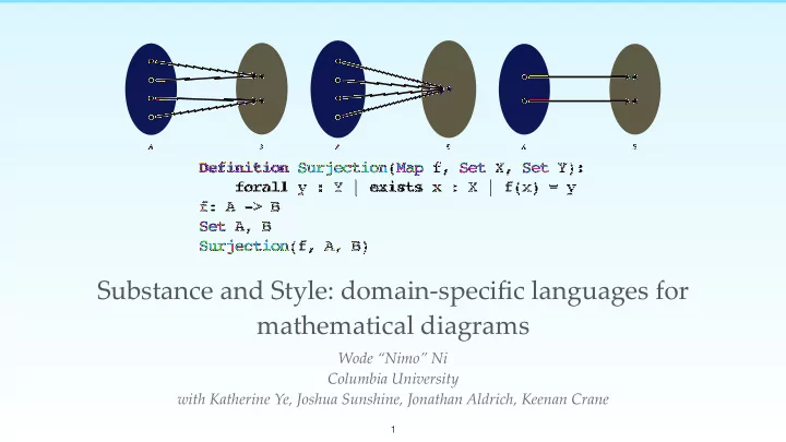
A B A B A B

Definition Surjection(Map f, Set X, Set Y): forall y : Y | exists x : X | f(x) = y f: A -> B Set A, B Surjection(f, A, B)

1
slide-2
SLIDE 2 Diagram from Wikipedia page for “sine”. h?ps://commons.wikimedia.org/wiki/File:Circle_cos_sin.gif 2
slide-3
SLIDE 3

Illustrating Venn diagram in TikZ

\documentclass{article} \usepackage{tikz} \begin{document} \pagestyle{empty} \begin{tikzpicture} \begin{scope}[shift={(3cm,-5cm)}, fill opacity=0.5] \draw[fill=red, draw = black] (0,0) circle (5); \draw[fill=green, draw = black] (-1.5,0) circle (3); \draw[fill=blue, draw = black] (1.5,0) circle (3); \node at (0,4) (A) {\large\textbf{A}}; \node at (-2,1) (B) {\large\textbf{B}}; \node at (2,1) (C) {\large\textbf{C}}; \node at (0,0) (D) {\large\textbf{D}}; \end{scope} \end{tikzpicture} \end{document} 3
slide-4
SLIDE 4

Illustrating Venn diagram in TikZ

\documentclass{article} \usepackage{tikz} \begin{document} \pagestyle{empty} \begin{tikzpicture}
  • 1. Specify the colors, sizes, and

locations of the circles

  • 2. Create “nodes” for the labels

and determine the locations of the labels

\end{tikzpicture} \end{document} 4
slide-5
SLIDE 5

Illustrating Venn diagram in TikZ

\documentclass{article} \usepackage{tikz} \begin{document} \pagestyle{empty} \begin{tikzpicture} \begin{scope}[shift={(3cm,-5cm)}, fill opacity=0.5] \draw[fill=red, draw = black] (0,0) circle (5); \draw[fill=green, draw = black] (-1.5,0) circle (3); \draw[fill=blue, draw = black] (1.5,0) circle (3); \node at (0,4) (A) {\large\textbf{A}}; \node at (-2,1) (B) {\large\textbf{B}}; \node at (2,1) (C) {\large\textbf{C}}; \node at (0,0) (D) {\large\textbf{D}}; \end{scope} \end{tikzpicture} \end{document} 5
slide-6
SLIDE 6

Illustrating Venn diagram in TikZ

\documentclass{article} \usepackage{tikz} \begin{document} \pagestyle{empty} \begin{tikzpicture} \begin{scope}[shift={(3cm,-5cm)}, fill opacity=0.5] \draw[fill=red, draw = black] (0,0) circle (5); \draw[fill=green, draw = black] (-1.5,0) circle (3); \draw[fill=blue, draw = black] (1.5,0) circle (3); \node at (0,4) (A) {\large\textbf{A}}; \node at (-2,1) (B) {\large\textbf{B}}; \node at (2,1) (C) {\large\textbf{C}}; \node at (0,0) (D) {\large\textbf{D}}; \end{scope} \end{tikzpicture} \end{document} 6

Low-level manipulation down to pixels. Semantics of the diagram is completely lost.

slide-7
SLIDE 7

Illustrating Venn diagram in TikZ

\documentclass{article} \usepackage{tikz} \begin{document} \pagestyle{empty} \begin{tikzpicture} \begin{scope}[shift={(3cm,-5cm)}, fill opacity=0.5] \draw[fill=red, draw = black] (0,0) circle (5); \draw[fill=green, draw = black] (-1.5,0) circle (3); \draw[fill=blue, draw = black] (1.5,0) circle (3); \node at (0,4) (A) {\large\textbf{A}}; \node at (-2,1) (B) {\large\textbf{B}}; \node at (2,1) (C) {\large\textbf{C}}; \node at (0,0) (D) {\large\textbf{D}}; \end{scope} \end{tikzpicture} \end{document} 7

What were we trying to illustrate

  • riginally?

Circles and text labels?

slide-8
SLIDE 8

Graph visualization using Graphviz

8

graph G { e subgraph clusterA { a -- b; subgraph clusterC { C -- D; } } subgraph clusterB { d -- f } d -- D e -- clusterB clusterC -- clusterB }

e a b C D d f
slide-9
SLIDE 9

Graph visualization using Graphviz

9 e a b C D d f

graph G { e subgraph clusterA { a -- b; subgraph clusterC { C -- D; } } subgraph clusterB { d -- f } d -- D e -- clusterB clusterC -- clusterB }

High-level and clean, but only works for graphs!

slide-10
SLIDE 10

Direct manipulation tools

10
slide-11
SLIDE 11

Penrose

11
slide-12
SLIDE 12

Language design

12
slide-13
SLIDE 13

Substance High-level declaration of mathematical objects

Set A, B Intersect A B Penrose has two extensible DSLs

Style Specifies the visual presentation

  • f the objects

Set A { shape = Circle{ } } Intersect X Y { ensure X overlapping Y }

13
slide-14
SLIDE 14 14

A B

Set A, B Intersect A B Set A { shape = Circle{ } } Intersect X Y { ensure X overlapping Y }

slide-15
SLIDE 15

Substance and Style

  • Power users encode domain expertise in Style
  • Casual users create diagrams declaratively using

Substance

Casual users Power users

15
slide-16
SLIDE 16
  • Dr. M wants to visualize a function…

How should I draw ?

16

f : X → Y

slide-17
SLIDE 17
  • Dr. M wants to visualize a function…

How should I draw ?

f: X -> Y

16

f : X → Y

slide-18
SLIDE 18
  • Dr. M wants to visualize a function…

How should I draw ?

f: X -> Y

16 Style file for functions Cartesian .sty Abstract .sty

f : X → Y

slide-19
SLIDE 19
  • Dr. M wants to visualize a function…

How should I draw f: X -> Y?

17
slide-20
SLIDE 20
  • Dr. M wants to visualize a function…
X Y f 18 Abstract .sty Cartesian .sty
slide-21
SLIDE 21

Style language

Selectors using pa?ern matching

Set X { shape = Circle { color = blue } }

19 C B A
slide-22
SLIDE 22

Style language

Cascading: later rules override the earlier ones

Set X { shape = Circle { color = blue } } Subset X Y { X.color = green }

20 C B A
slide-23
SLIDE 23

Style language Set X { shape = Circle { color = blue } } Subset X Y { X.color = green } Set `A` { A.color = pink }

21 C B A
slide-24
SLIDE 24

Style language

  • Wait. How does Penrose choose

the positions and sizes of them?

22

Set X { shape = Circle { color = blue } } Subset X Y { X.color = green } Set `A` { A.color = pink }

C B A
slide-25
SLIDE 25

Style language

23
  • Wait. How does Penrose choose

the positions and sizes of them?

Set X { shape = Circle { color = blue } } Subset X Y { X.color = green } Set `A` { A.color = pink }

C B A
slide-26
SLIDE 26

Optimization-based layout

24
slide-27
SLIDE 27

Specifying Layout in Style

Set X { shape = Circle { color = blue } }

Subset X Y { X.color = green }

ensure X contains X.label ensure Y contains X ensure X smallerThan Y ensure Y.label outsideOf X

Declaratively specify

  • ptimization requirements!
25 C B A
slide-28
SLIDE 28

Optimizing diagram layout

Energy Time

26
slide-29
SLIDE 29

Optimizing diagram layout

Energy Time

A B C D E F G A B C D E F G A B C D E F G A B C D E F G 27

Exterior point method + line search

slide-30
SLIDE 30

Illustrating abstract function definitions

28
slide-31
SLIDE 31

Injective functions

∀x, x0 ∈ X, f(x) = f(x0) → x = x0.

A function is injective, or “one-to-one,” if every element

  • f its codomain is mapped from at most one element of the

domain.

29

Definition Injection(Map f, Set A): forall a1, a2 : A | f(a1) = f(a2) implies a1 = a2

slide-32
SLIDE 32

Extend with external tools

  • Penrose doesn’t have to understand first order logic!
  • Extend the system to integrate with an external tool, Alloy, to

generate concrete instances given the definition of injective functions.

30 Definition Injection(Map f, Set A): forall a1, a2 : A | f(a1) = f(a2) implies a1 = a2 f: A -> B Set A, B Injection(f, A)

Penrose program

slide-33
SLIDE 33

Extend with external tools

  • Penrose doesn’t have to understand first order logic!
  • Extend the system to integrate with an external tool, Alloy, to

generate concrete instances given the definition of injective functions.

30 Definition Injection(Map f, Set A): forall a1, a2 : A | f(a1) = f(a2) implies a1 = a2 f: A -> B Set A, B Injection(f, A)

Penrose program

slide-34
SLIDE 34

Extend with external tools

  • Penrose doesn’t have to understand first order logic!
  • Extend the system to integrate with an external tool, Alloy, to

generate concrete instances given the definition of injective functions.

30
slide-35
SLIDE 35

Extend with external tools

  • Penrose doesn’t have to understand first order logic!
  • Extend the system to integrate with an external tool, Alloy, to

generate concrete instances given the definition of injective functions.

30

sig A { f : B } sig B { } fact { all a1,a2 : A | a1.f = a2.f implies a1 = a2 } pred show() { } run show for 5

All

slide-36
SLIDE 36

Extend with external tools

  • Penrose doesn’t have to understand first order logic!
  • Extend the system to integrate with an external tool, Alloy, to

generate concrete instances given the definition of injective functions.

30 sig A { f : B } sig B { } fact { all a1,a2 : A | a1.f = a2.f implies a1 = a2 } pred show() { } run show for 5

All

slide-37
SLIDE 37

Extend with external tools

  • Penrose doesn’t have to understand first order logic!
  • Extend the system to integrate with an external tool, Alloy, to

generate concrete instances given the definition of injective functions.

30 sig A { f : B } sig B { } fact { all a1,a2 : A | a1.f = a2.f implies a1 = a2 } pred show() { } run show for 5

All

A: {A$0} B: {B$0, B$1, B$2, B$3, B$4} f: {A$0->B$4}

Alloy instances

slide-38
SLIDE 38

Extend with external tools

  • Penrose doesn’t have to understand first order logic!
  • Extend the system to integrate with an external tool, Alloy, to

generate concrete instances given the definition of injective functions.

30
slide-39
SLIDE 39

Extend with external tools

31 B A
  • Penrose doesn’t understand first order logic!
  • Extend the system to integrate with an external tool, Alloy, to

generate concrete instances given the definition of injective functions.

slide-40
SLIDE 40

Visualizing injective functions

B A 32
slide-41
SLIDE 41

Visualizing injective functions

B A B A 32
slide-42
SLIDE 42

Visualizing injective functions

B A B A B A 32
slide-43
SLIDE 43

Visualizing injective functions

B A B A B A

A bijection is a special case of injection!

32
slide-44
SLIDE 44

Visualizing composition of functions

C B A f g C B A f g

Set A, B, C f: A -> B g: B -> C Injection(f, A) Injection(g, B)

33
slide-45
SLIDE 45

Visualizing composition of functions

C B A f g C B A f g

Set A, B, C f: A -> B g: B -> C Injection(f, A) Injection(g, B)

The composition of injections is still an injection!

33
slide-46
SLIDE 46

Running Penrose

34
slide-47
SLIDE 47

Example: Venn vs Tree diagram

Set A, B, C, D, E, F, G Subset B A Subset C A Subset D B Subset E B Subset F C Subset G C NoIntersect E D NoIntersect F G NoIntersect B C

35
slide-48
SLIDE 48

Example: Venn vs Tree diagram

36
slide-49
SLIDE 49

Example: Venn vs Tree diagram

36
slide-50
SLIDE 50

Example: restarting the optimization

37
slide-51
SLIDE 51

Conclusion

  • Goal: Enables users to make

beautiful diagrams without design background

  • DSLs that cleanly separate

high-level semantics and styling details

  • Optimizes layout declaratively
  • Extensible system

http://penrose.ink http://github.com/penrose/penrose

A B A B C D E F G A B C D E F G B R1 R2 U V f A 38